Quick start — fit your first covariance ellipse

Goal: run the full psyphy workflow — simulate data, fit a model, inspect the result — in one short script with no GPU required.

The complete runnable script is quick_start.py. For a spatially-varying field over a 2-D stimulus grid, see the full example.

---

Runtime

Hardware	Approximate time
GPU (any modern CUDA device)	< 5 s
CPU (laptop / M-series Mac)	< 1 min

The three knobs that control runtime:

MC_SAMPLES = 50  # MC samples per trial in the likelihood (full example: 500)
NUM_TRIALS = 100  # total simulated trials (full example: 4000 × 25)
NUM_STEPS = 200  # optimizer steps (full example: 2000)

learning_rate = 5e-4  # full example: 5e-5. The smaller the lr, the more steps
# are required.

---

Step 0 — Imports

from psyphy.data import TrialData  # batched trial container
from psyphy.inference import MAPOptimizer  # fitter
from psyphy.model import (
    WPPM,
    GaussianNoise,
    OddityTask,
    OddityTaskConfig,
    Prior,
    WPPMCovarianceField,  # fast Σ(x) evaluation
)

---

Step 1 — Define a ground-truth model and sample parameters

We create a WPPM with known parameters to act as the synthetic observer. Data will be generated from it so we have a ground truth to compare against.

task = OddityTask(config=OddityTaskConfig(num_samples=int(MC_SAMPLES)))
noise = GaussianNoise(sigma=0.1)

# Set all Wishart process hyperparameters in Prior
truth_prior = Prior()
truth_model = WPPM(
    prior=truth_prior,
    likelihood=task,
    noise=noise,
)

# Sample ground-truth Wishart process weights
truth_params = truth_model.init_params(jax.random.PRNGKey(123))

---

Step 2 — Simulate trials at a single reference point

We generate NUM_TRIALS oddity-task responses at a single reference stimulus ref = [0, 0]. Probe displacements are scaled by the local covariance (constant Mahalanobis radius), so trial difficulty stays roughly uniform.

# Simulate observed responses using the likelihood implied by the task
ys, p_correct = task.simulate(truth_params, refs, comparisons, truth_model, key=k_sim)

The TrialData container is the canonical input for fitting:

data = TrialData(
    refs=refs, comparisons=comparisons, responses=ys
)  # contains 3 JAX arrays

---

Step 3 — Build the model to fit

We build a fresh WPPM with the same hyperparameters but independent random weights, then take one draw from the prior as the starting point for optimization.

prior = Prior()

model = WPPM(
    prior=prior,
    likelihood=task,
    noise=noise,  # we use the same Gaussian noise as for the ground truth
)

# Initialize parameters at a sample from the prior
init_params = model.init_params(
    jax.random.PRNGKey(42)
)  # intitialize with a draw from the prior
prior_field = WPPMCovarianceField(model, init_params)
# Evaluate prior covariance at the reference point
covs_prior = prior_field(ref_point)  # (1, 2, 2)

---

Step 4 — Fit with MAP optimization

inference = MAPOptimizer(
    steps=NUM_STEPS,
    learning_rate=learning_rate,
    track_history=True,
    log_every=1,
)

map_estimate = inference.fit(model, data, init_params=init_params, seed=4)
# Protocol: ParameterPosterior, here point estimate

# optional: for visualization:
map_cov_field = WPPMCovarianceField(model, map_estimate.params)
# OUTPUT: Covariance Matrices (N, 2, 2) for plotting

MAPOptimizer runs SGD + momentum and returns a MAPPosterior — a point estimate at \(W_\text{MAP}\).

---

Step 5 — Inspect the fitted covariance ellipse

WPPMCovarianceField binds a (model, params) pair into a single callable that returns \(\Sigma(x)\) for any stimulus x:

# Evaluate any covariance-field object at a single point or a batch of points.
covs_truth = truth_field(ref_point)  # (N, 2, 2)
covs_prior = prior_field(ref_point)  # (N, 2, 2)
covs_map = map_cov_field(ref_point)  # (N, 2, 2)
# here: N=1 for fast computation

The ellipse plot below overlays the ground truth (black), the prior initialization (blue), and the MAP fit (red) at the single reference point:

_PLOT_JITTER = 0.0


# Evaluate any covariance-field object at a single point or a batch of points.
covs_truth = truth_field(ref_point)  # (N, 2, 2)
covs_prior = prior_field(ref_point)  # (N, 2, 2)
covs_map = map_cov_field(ref_point)  # (N, 2, 2)
# here: N=1 for fast computation

# Scale ellipses so they are visually readable.
gt_scale = float(jnp.sqrt(jnp.mean(jnp.linalg.eigvalsh(covs_truth[0]))))
ellipse_scale = max(0.3, 0.4 * gt_scale / 0.01)  # keep readable on the unit square

fig, ax = plt.subplots(figsize=(6, 6))

labels = ["Ground Truth", "Prior Sample (init)", "Fitted (MAP)"]
colors = ["k", "b", "r"]
fields = [truth_field, prior_field, map_cov_field]
non_pd_counts = []

for field, color, label in zip(fields, colors, labels):
    covs = field(ref_point)
    segments, valid = _ellipse_segments_from_covs(
        ref_point,
        covs,
        scale=ellipse_scale,
        plot_jitter=_PLOT_JITTER,
        unit_circle=_UNIT_CIRCLE,
    )
    non_pd_counts.append(int((~valid).sum()))
    lc = LineCollection(
        jax.device_get(segments),
        colors=color,
        linewidths=2.0,
        alpha=0.8,
    )
    ax.add_collection(lc)
    ax.plot([], [], color=color, alpha=0.8, linewidth=1.5, label=label)

ax.scatter(
    ref_point[:, 0], ref_point[:, 1], c="g", s=40, zorder=5, label="Reference Point"
)
ax.set_xlim(-0.6, 0.6)
ax.set_ylim(-0.6, 0.6)
ax.set_aspect("equal", adjustable="box")
ax.set_xlabel("Stimulus dimension 1")
ax.set_ylabel("Stimulus dimension 2")
ax.set_title(
    f"Covariance ellipse at ref={ref_point[0].tolist()}\n"
    f"lr={learning_rate}, steps={NUM_STEPS}, MC-samples={MC_SAMPLES}, trials={NUM_TRIALS}"
)
ax.grid(True, alpha=0.3)
ax.legend(loc="upper right")
plt.tight_layout()

os.makedirs(PLOTS_DIR, exist_ok=True)
fig.savefig(
    os.path.join(PLOTS_DIR, "quick_start_ellipses.png"), dpi=200, bbox_inches="tight"
)
print(f"  Saved → {PLOTS_DIR}/quick_start_ellipses.png")

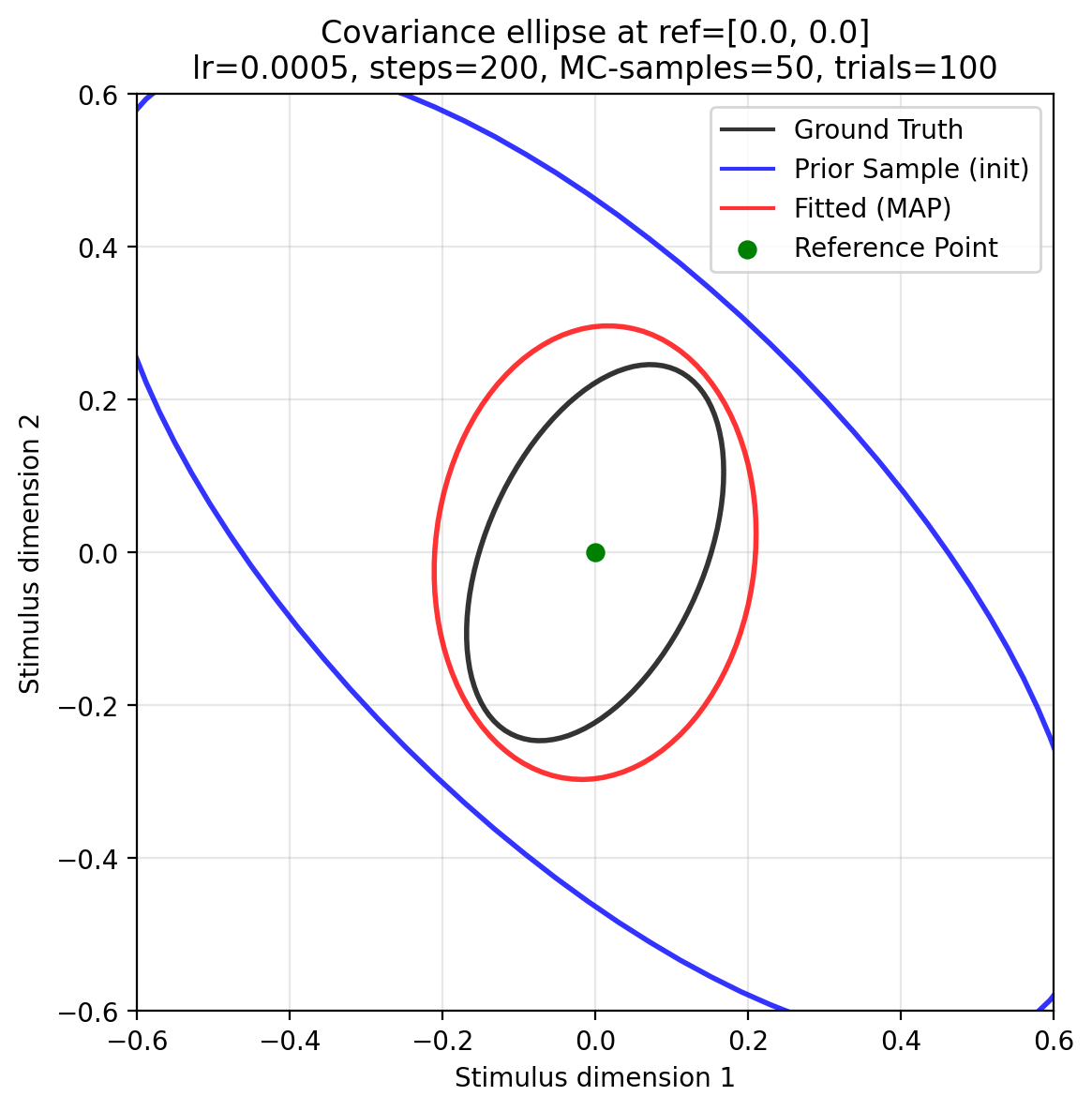
Ground truth (black), prior sample (blue), and MAP-fitted (red) covariance ellipses at the single reference point. Note how the red ellipse has moved from the blue (init) closer to the ground truth (black).

---

Step 6 — Learning curve

steps_hist, loss_hist = inference.get_history()

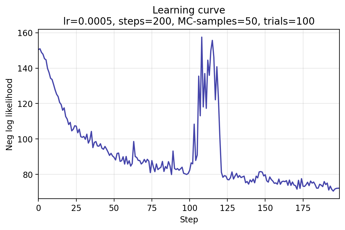
Negative log-likelihood over optimizer steps.

---

Next steps

• Spatially-varying field: scale up to a full 2-D grid → full example.
• Your own data: replace the simulated TrialData with your own refs, comparisons, and responses arrays.
• API reference: see MAPOptimizer, WPPM, and WPPMCovarianceField.