NUTS Posterior Inference for WPPM¶

This tutorial demonstrates full posterior inference using the No-U-Turn Sampler (NUTS) for the Wishart Process Psychophysical Model (WPPM).

The companion script can be found at nuts_inference_example.py.

How to run the script

An install of psyphy on its own is not enough. This page needs three optional dependencies, none of which psyphy requires by default.

pip install 'psyphy[sampling,diagnostics,viz]'

extra	brings in	what it is for
`sampling`	`blackjax>=1.4,<2`	`NUTSSampler` itself
`diagnostics`	`arviz>=1.0`	`MCMCPosterior.to_arviz()`, R-hat, ESS, the trace plot
`viz`	`matplotlib>=3.5`	every figure on this page

Everything on this page comes from one script. Pick a preset by how much compute you want to spend:

# smoke test: 9 refs, 50 MC samples, 2 chains x (100 warmup + 150 draws)
python nuts_inference_example.py --mode quick

# 25 refs, 500 MC samples, 4 chains x (500 + 500). Minutes on a GPU.
python nuts_inference_example.py --mode balanced

# 25 refs, 2000 MC samples, 4 chains x (1000 + 1000). Wants a GPU.
python nuts_inference_example.py --mode full

quick exists so the page can be regenerated on a GPU within 2 minutes. Its diagnostics are deliberately not publication grade; see Step 5.

Background: why MCMC, and what it is¶

MAP estimation returns a single point estimate \(\theta_\text{MAP}\):

\[\theta_\text{MAP} = \arg\max_\theta \left[\log p(\mathcal{D} \mid \theta) + \log p(\theta)\right]\]

This tells you where the posterior peaks, but not how wide it is. If the data are sparse or ambiguous the posterior may be broad, and the MAP estimate alone cannot tell you that. For a threshold contour the difference is the whole point: a point estimate gives one curve, where what you want to report is a curve with a band around it.

What we actually want instead is the posterior \(p(\theta \mid \mathcal{D})\), the full distribution over parameters given the data. Bayes' rule writes it down in one line, but the line contains an integral over all of parameter space that nobody can evaluate here: W has 54 entries in the smallest setting on this page. We cannot plot the posterior, and we cannot integrate against it directly.

Markov chain Monte Carlo sidesteps that. Instead of computing the distribution, you construct a random walk whose long-run visiting frequency is that distribution. Run it long enough and the places it has been form a sample from the posterior, which is all you need: averages over the sample approximate averages over the posterior, and the spread of the sample is the uncertainty. Nothing is ever normalised, which is the trick, because the intractable integral is exactly the normalising constant.

The catch is building a walk that explores efficiently. A naive random walk works in two or three dimensions and fails badly in fifty, where almost every direction you could step in leads somewhere less probable, so nearly all proposals are rejected and the chain crawls. Hamiltonian Monte Carlo fixes this by using the gradient of the log posterior: it gives the parameter vector a random momentum and simulates it rolling along the posterior's own geometry, so a single proposal can travel a long way and still be accepted. NUTS, the No-U-Turn Sampler of Hoffman and Gelman (2014), removes the one awkward tuning knob by extending each trajectory until it starts to double back on itself. Betancourt's Conceptual Introduction to Hamiltonian Monte Carlo is the readable account of why this works and where it fails; it is worth an hour if you intend to trust these numbers.

Two things follow for psyphy, and both shape this page:

The sampler needs gradients, which is why the log posterior is written in JAX and why NUTSSampler can hand it straight to BlackJAX.
The sampler needs the log density to be a fixed function. psyphy's oddity likelihood is estimated by Monte Carlo simulation, so it is not fixed; it returns a slightly different number each call. That tension is real, and the determinism note below explains what is done about it.

What you get in exchange for the extra compute:

Uncertainty quantification: how spread out is our belief over model parameters?
Posterior predictive distributions: how uncertain are our predictions at new test points?
Convergence diagnostics: unlike optimisation, MCMC can tell you when it has failed.

The posterior predictive distribution¶

Given posterior samples \(\theta_i \sim p(\theta \mid \mathcal{D})\), predictions at new test points \(X^*\) are:

\[p(\text{correct} \mid X^*, \mathcal{D}) = \int p(\text{correct} \mid X^*, \theta)\; p(\theta \mid \mathcal{D})\; d\theta \approx \frac{1}{N} \sum_{i=1}^{N} \underbrace{p(\text{correct} \mid X^*, \theta_i)}_{\texttt{OddityTask.predict}(\theta_i,\, X^*)}\]

In psyphy this is computed by WPPMPredictivePosterior, which calls nuts_posterior.sample(N) to get \(N\) parameter draws and vmaps the task likelihood over them. The same class works identically with a MAPPosterior (which just returns \(N\) copies of \(\theta_\text{MAP}\)).

A note on the likelihood¶

In this tutorial, we use the MC-based likelihood which is estimated via Monte Carlo inside OddityTask.loglik and expensive.

Future Alternatives - Neural surrogate likelihood: replace the MC estimator with a trained neural network for exact gradients (see NeuralSurrogateTask).

Step-by-step walkthrough¶

Step 1: Simulate data¶

Same setup as the full MAP example. Data is a TrialData object:

Simulated data
data = TrialData(stimuli=stimuli, responses=ys)

Step 2: Build the model¶

Model definition
prior = Prior(
    input_dim=INPUT_DIM,
    basis_degree=BASIS_DEGREE,
    extra_embedding_dims=EXTRA_DIMS,
    decay_rate=DECAY_RATE,
    variance_scale=VARIANCE_SCALE,
)
model = WPPM(
    input_dim=INPUT_DIM,
    prior=prior,
    likelihood=task,
    noise=noise,
    diag_term=DIAG_TERM,
)

Step 3: MAP warm-start (recommended)¶

Starting NUTS near the posterior mode dramatically reduces the warmup needed. Run a short MAP fit first:

MAP warm-start
map_optimizer = MAPOptimizer(
    steps=MAP_STEPS,
    learning_rate=MAP_LR,
    momentum=MAP_MOMENTUM,
    track_history=True,
    show_progress=True,
)
map_posterior = map_optimizer.fit(model, data, seed=SEED)

Then pass map_posterior.params as init_params to NUTSSampler.fit().

Step 4: NUTS sampling¶

NUTS sampling with NUTSSampler
sampler = NUTSSampler(
    num_warmup=NUM_WARMUP,
    num_samples=NUM_SAMPLES,
    num_chains=NUM_CHAINS,
    logdensity_key_seed=0,  # fixed MC key → deterministic Hamiltonian
    target_acceptance_rate=0.8,
    max_num_doublings=MAX_NUM_DOUBLINGS,  # cap: <= 255 grad evals per draw
    # Sample z = W / prior_std so warmup starts from a metric matched to the
    # prior scales instead of the identity (the default; shown for clarity).
    prior_preconditioning=True,
    show_progress=True,
)
nuts_posterior = sampler.fit(
    model,
    data,
    init_params=map_posterior.params,  # warm-start from MAP
    seed=7,
)

NUTSSampler has the same fit(model, data) interface as MAPOptimizer; the BlackJAX backend is entirely hidden. It returns an MCMCPosterior satisfying the same ParameterPosterior protocol as MAPPosterior.

Compute settings. The script takes --mode, which selects a preset. The model is identical in every mode, so only the thoroughness of the fit changes, never what is being fit:

python nuts_inference_example.py                    # quick (default): GPU smoke test (3 min)
python nuts_inference_example.py --mode balanced    # a real fit, roughly a GPU-hour
python nuts_inference_example.py --mode full        # paper-scale MC, 4 x 1000 draws

# Compute/fidelity presets. Same MODES convention as hong2025_reproduction.py.
#
# Why each knob is where it is in `full`:
#   mc_samples 2000  the value hong2025.PAPER_HYPERPARAMS uses for this model
#                    class. It is the knob that matters most here: the MC
#                    likelihood is only deterministic because NUTSSampler
#                    freezes one PRNG key, which makes the sampled posterior
#                    the one implied by that noise draw. The bias shrinks as
#                    mc_samples grows -- 50 is a smoke test, 200 the documented
#                    minimum, 2000 the paper's.
#   trials 5000      25 reference points x 200 trials. 450 trials (quick) is
#                    thin for this many coefficients, and under-determined
#                    posteriors are wide for reasons that have nothing to do
#                    with the sampler.
#   4 x 1000 draws   the standard NUTS configuration, and what the shapes in
#                    the design note assume. R-hat needs >= 2 chains (4 is
#                    convention) and ESS > 100 per parameter needs the draws.
#   warmup 1000      dual averaging tunes the step size AND the mass matrix;
#                    for WPPM the mass matrix matters a lot, because
#                    coefficients at different Chebyshev degrees have genuinely
#                    different prior scales. 100 warmup steps cannot do it.
MODES = {
    "quick": {
        "mc_samples": 50,
        "trials_per_ref": 50,
        "n_ref_grid": 3,
        "map_steps": 300,
        "warmup": 100,
        "draws": 150,
        "chains": 2,
        "ensemble": 30,
    },
    "balanced": {
        "mc_samples": 500,
        "trials_per_ref": 100,
        "n_ref_grid": 5,
        "map_steps": 800,
        "warmup": 500,
        "draws": 500,
        "chains": 4,
        "ensemble": 100,
    },
    "full": {
        "mc_samples": 2000,
        "trials_per_ref": 200,
        "n_ref_grid": 5,
        "map_steps": 1500,
        "warmup": 1000,
        "draws": 1000,
        "chains": 4,
        "ensemble": 200,
    },
}

Runtime notes

The MC likelihood dominates everything. Each gradient evaluation simulates mc_samples Monte Carlo draws for every trial, so cost scales with mc_samples × n_trials. Going from quick to full raises that product by ~440×, which is why full is a batch job and not something to run interactively.
NUTS cost per draw is not fixed. It is O(2^tree_depth) gradient evaluations, and the depth is data-dependent, commonly 16 to 64 evaluations per draw. The script therefore times one gradient and prints a bracketed projection before sampling starts, so you can see whether a run fits inside a Slurm time limit before committing to it.
Tree depth is capped. NUTSSampler(max_num_doublings=8) (the default) limits a draw to at most 2^8 − 1 = 255 gradient evaluations; BlackJAX's own default of 10 allows 1023. If sampler_stats["n_steps"] sits at the cap for most draws, trajectories are being truncated: still valid MCMC, but slower mixing. Raise the cap or reparameterize.
Warmup starts from a prior-scaled metric. By default the sampler works in z = W / prior_std (prior_preconditioning=True), so adaptation does not begin from an identity mass matrix that is badly mismatched to coefficients whose scales span 0.06 to 0.01. Without this, early warmup runs every draw to the maximum tree depth.
Chains are vmapped, in both warmup modes. All chains advance in one compiled call per phase, so XLA compiles once rather than once per chain. Under vmap each step costs as much as the deepest tree across chains, which is one more reason for the depth cap. Note: the progress bar moves only when each phase (warmup, sampling) finishes.

Two warmup modes¶

Mode	When	How
Adaptive (default, `step_size=None`)	Best quality; adapts step size and mass matrix per chain via `blackjax.window_adaptation`, starting from a prior-scaled metric. Chains vmapped; each adapts independently.	`NUTSSampler(num_warmup=200, num_samples=500)`
Fixed (`step_size=<float>`)	Faster with many chains; no adaptation. All chains vmapped in one compiled call. User must choose a good step size.	`NUTSSampler(..., step_size=0.01)`

Step 5: Diagnostics with ArviZ¶

Sampling gives you draws; it does not tell you whether to trust them. MCMC fails quietly, so a chain can look like a result while having explored only part of the posterior. ArviZ is the standard Python library for that check. It is backend-agnostic, so the same diagnostics apply whether the draws came from BlackJAX, NumPyro, Stan or PyMC.

psyphy hands your chains over in one call:

idata = nuts_posterior.to_arviz()

to_arviz() converts the (n_chains, n_draws, *W_shape) arrays, plus the sampler statistics, into ArviZ's format. No reshaping is needed; ArviZ handles arbitrary-rank variables natively and computes diagnostics per scalar element of W. Everything ArviZ offers is then available on idata.

ArviZ diagnostics
idata = nuts_posterior.to_arviz()
summary = az.summary(idata, var_names=["W"])
print(summary[["mean", "sd", "r_hat", "ess_bulk"]].describe())
r_hat_max = float(summary["r_hat"].max())
ess_min = float(summary["ess_bulk"].min())
print(f"  R-hat max: {r_hat_max:.3f}  (target < 1.01)")
print(f"  ESS min:   {ess_min:.0f}    (target > 100 per chain)")

Trace plot
pc = az.plot_trace(
    idata,
    var_names=["W"],
    coords={"W_dim_2": 0, "W_dim_3": 0},
    col_wrap=3,
    visuals={"xlabel": False},
)
# Reaching into arviz_plots internals for the caption: cosmetic only
with contextlib.suppress(Exception):
    pc.viz["figure"].item().suptitle(
        "Posterior traces for W[deg_x, deg_y, 0, 0]. 1 panel per Chebyshev "
        "coefficient\ncolours = chains · x = draw index (post-warmup)",
        fontsize=10,
    )
pc.savefig(plot_path("nuts_trace_plot.png"))

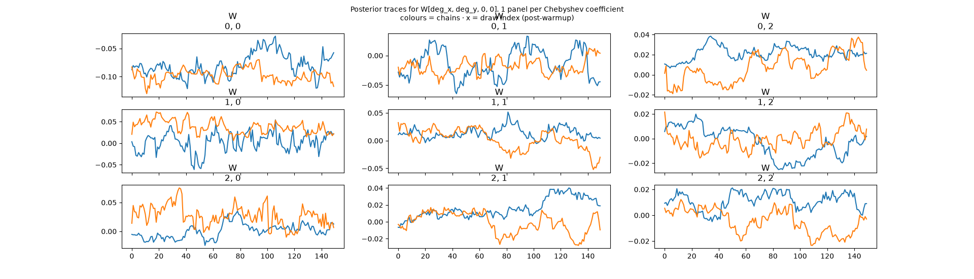
Posterior traces for the slice W[:, :, 0, 0].

How to read it. W has shape (3, 3, 2, 3) = (deg_x, deg_y, U_row, U_col): the first two axes index the Chebyshev basis, giving degree along stimulus dimension 1 and along dimension 2. The last two index the entry of U(x), where Σ = U Uᵀ + diag_term·I. That is 54 scalars, past ArviZ's plot.max_subplots limit and illegible anyway, so the figure fixes U[0, 0] and plots the remaining 3×3 coefficient grid, laid out as that grid by col_wrap=3.

element of the figure	what it is
one panel	one Chebyshev coefficient; the title `i, j` is degree `i` × degree `j`
x axis	draw index within a chain, post-warmup (warmup draws are discarded, not plotted)
y axis	the value of that coefficient
one coloured line per panel	one chain
black ticks along the bottom	divergences; they appear because `sampler_stats` carries `diverging` under ArviZ's standard name

What good looks like: chains overlapping each other, flat, and wiggling fast, the "fuzzy caterpillar". A chain that drifts steadily across the panel has not converged: warmup was too short and the sampler is still finding the typical set. That is the single most common thing this plot catches, and it is a reason to raise --mode, not a reason to distrust the model.

It is generated by ArviZ, from MCMCPosterior.to_arviz(); no psyphy plotting code is involved. On ArviZ ≥ 1.0 plot_trace returns an arviz_plots PlotCollection (not an array of matplotlib axes), so it is saved with pc.savefig(); the 0.x kwargs compact= and figsize= no longer exist and raise if passed. For the classic density-plus-trace pairing, ArviZ 1.x has a separate az.plot_trace_dist.

Interpreting diagnostics¶

The 4 most important Diagnostics:

Diagnostic	What it measures	Good value
Divergences	Transitions where the integrator blew up, usually in a region of high curvature the step size cannot resolve.	0. Any divergence makes the run suspect, whatever R-hat says.
R-hat	Between-chain variance over within-chain variance; near 1 means the chains agree on the same distribution.	< 1.01
ESS (bulk)	Effective sample size: how many independent draws the chains are worth once autocorrelation is accounted for.	> 100 per chain
Acceptance rate	Fraction of NUTS proposals accepted. Far below target means the step size is too large; far above means it is inefficiently small.	0.6 to 0.9

Divergences come first, because the other three can all look healthy while the sampler is systematically missing part of the posterior. A divergence means the simulated trajectory blew up rather than following the posterior's geometry, which usually points at a region of curvature the step size cannot resolve, and the draws you keep are then biased in a way no amount of extra sampling fixes. Betancourt's Conceptual Introduction is the place to read what they mean geometrically. psyphy records them for you: sampler_stats carries diverging, energy and n_steps under ArviZ's standard names, so az.plot_energy(idata) and the divergence ticks on the trace plot work with no extra wiring.

R-hat compares chains against each other, so it needs at least two of them; a single chain cannot tell you it is stuck. The idea goes back to Gelman and Rubin (1992), but the version ArviZ computes is the rank-normalized, split variant of Vehtari et al. (2021), which is also where the < 1.01 and > 100 thresholds above come from. They are recommendations from that paper rather than folklore, and the paper is worth skimming for why the older < 1.1 rule of thumb turned out to be too lenient.

With --mode quick (2 chains and 150 draws) R-hat and ESS will not reach these thresholds, and they are not meant to. Use --mode balanced or --mode full, which exist for exactly this reason, before drawing any conclusion from the numbers.

Step 6: Posterior predictive uncertainty¶

Draw posterior parameter samples
n_ensemble = N_ENSEMBLE
param_samples = nuts_posterior.sample(n_ensemble, key=jr.PRNGKey(0))
# param_samples["W"].shape == (n_ensemble, *W_shape)

Plot ensemble of ellipses
# The posterior spread, drawn first so it sits behind the two lines. One call:
# (n_ensemble, n_ref, 2, 2) is the "several fields" shape plot_ellipses takes.
plot_ellipses(
    jax.device_get(ref_points),
    jax.device_get(ensemble_covs(param_samples, ref_points)),
    ax=ax,
    scale=ELLIPSE_SCALE,
    colors="#4444cc",
    linewidths=0.5,
    alpha=0.15,
)

# Posterior mean and ground truth, overlaid as a list of fields so each gets its
# own colour, width and legend entry.
plot_ellipses(
    jax.device_get(ref_points),
    [jax.device_get(covs_mean), jax.device_get(covs_truth)],
    ax=ax,
    scale=ELLIPSE_SCALE,
    colors=["#cc2222", "k"],
    labels=["Posterior mean", "Ground truth"],
    linewidths=[1.5, 1.2],
    alpha=[0.9, 0.7],
)

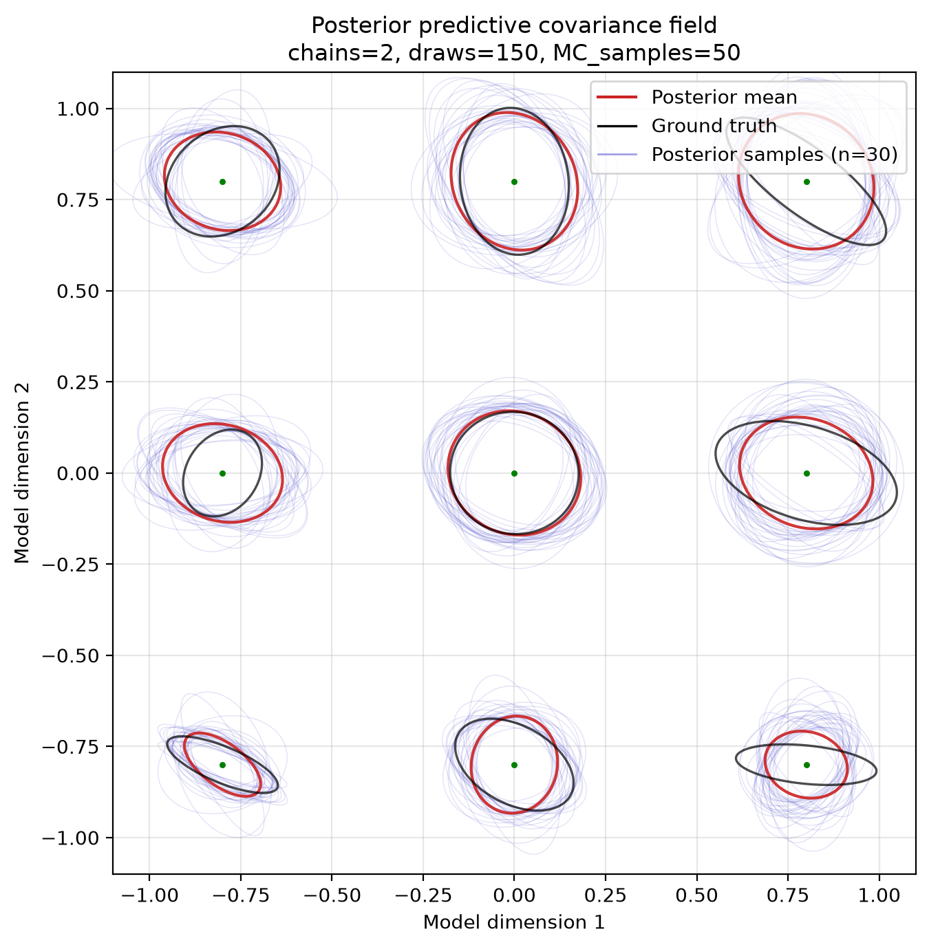
Faint blue: 30 covariance fields sampled from the posterior. Red: posterior mean. Black: ground truth. The spread of blue ellipses shows where the model is uncertain.

Step 7: MAP vs NUTS comparison¶

The asymmetry between the panels is the point. MAP can only ever draw one contour, because its posterior is a delta at θ_MAP: MAPPosterior.sample(n) returns θ_MAP repeated n times, so the ensemble it produces has zero spread. NUTS puts a band around the same contour, from identical downstream code. WPPMPredictivePosterior never asks which kind of posterior it was given. Plotting only the two means would make them look like equivalent point estimates and lose the one thing full posterior inference buys you.

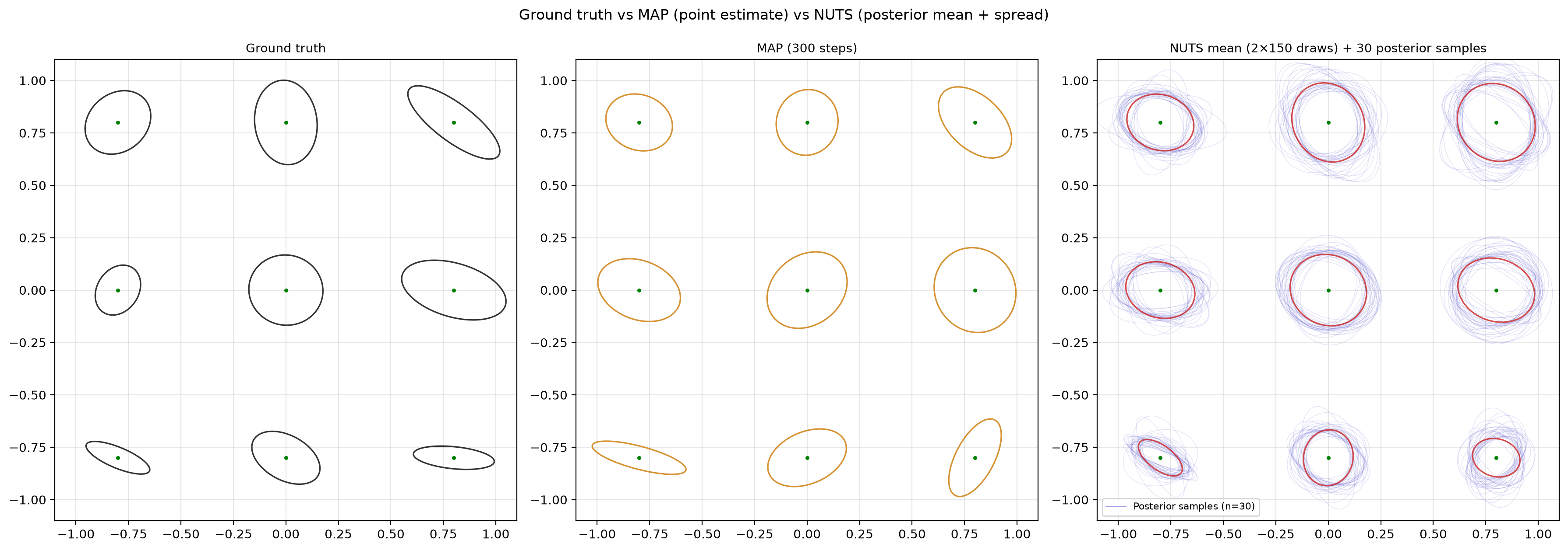
Ground truth (left), MAP point estimate (centre), NUTS posterior mean with its posterior sample ensemble in faint blue (right).

Step 8: Everything in one axes¶

Side-by-side panels make you compare from memory. This figure puts all four layers on one set of axes so the disagreements can be read off directly: where the posterior band covers the ground truth, the fit is honest about what it does not know; where the truth falls outside the band, the model is confidently wrong, and no amount of extra draws will fix it.

Overlay with psyphy.viz
# Posterior spread first, so it sits behind the three lines.
fig, ax = plt.subplots(figsize=(8, 8))
plot_ellipses(
    jax.device_get(ref_points),
    ensemble,
    ax=ax,
    scale=ELLIPSE_SCALE,
    colors="#4444cc",
    linewidths=0.5,
    alpha=0.15,
)
plot_ellipses(
    jax.device_get(ref_points),
    [
        jax.device_get(truth_field(ref_points)),
        jax.device_get(WPPMCovarianceField(model, map_posterior.params)(ref_points)),
        jax.device_get(covs_mean),
    ],
    ax=ax,
    scale=ELLIPSE_SCALE,
    colors=["k", "#cc7700", "#cc2222"],
    labels=["Ground truth", f"MAP ({MAP_STEPS} steps)", "NUTS posterior mean"],
    linewidths=[1.2, 1.4, 1.6],
    linestyles=["-", "--", "-"],
    alpha=[0.8, 0.9, 0.95],
    show_centers=True,
)

Every ellipse here is drawn by psyphy.viz

All three covariance figures on this page go through plot_ellipses, which accepts the covariances in whichever shape you already have:

shape	meaning
`(n_points, 2, 2)`	one field, for instance the posterior mean
list of `(n_points, 2, 2)`	several fields overlaid, each with its own colour, width, linestyle and legend entry
`(n_samples, n_points, 2, 2)`	a stack of fields, which is exactly what `sample()` returns

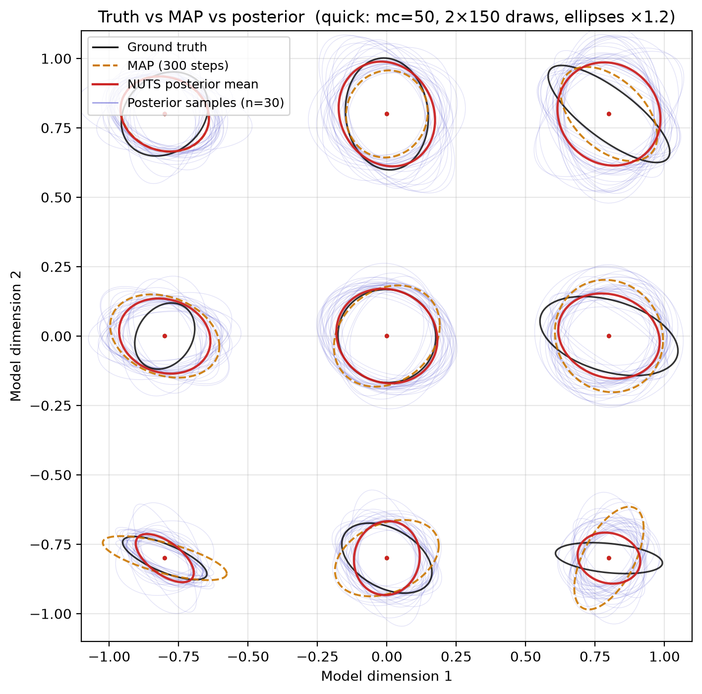
Faint blue: posterior draws. Black: ground truth. Dashed orange: MAP. Red: posterior mean. All at the same ELLIPSE_SCALE as the figures above, so the three are comparable.

scale and honest ellipse sizes

Every figure on this page multiplies the ellipses by ELLIPSE_SCALE so they are visible against the grid; they are not drawn at true size. plot_ellipses also accepts scale="auto", which sizes the median ellipse to a fraction of the grid spacing and can return the factor it used via return_scale=True, so a figure can report its own magnification.

Architecture recap¶

NUTSSampler.fit(model, data)        <- same interface as MAPOptimizer
        ↓  returns
MCMCPosterior                        <- satisfies ParameterPosterior protocol
  .params        → posterior mean W
  .sample(n,key) → n draws {"W": (n, *W_shape)}
  .to_arviz()    → xarray.DataTree (n_chains, n_draws, *W_shape)
        ↓
WPPMPredictivePosterior(nuts_posterior, X_test, ...)
  .mean     → E[p(correct | X*, θ) | D]
  .variance → Var[p(correct | X*, θ) | D]

WPPMPredictivePosterior is permanently agnostic about whether it wraps a MAPPosterior or MCMCPosterior; the ParameterPosterior protocol is the firewall.

Limitations and future extensions¶

Fixed MC key bias: the MC oddity likelihood is stochastic, and BlackJAX needs a deterministic log density, so one PRNG key is frozen into the closure. That fixes the noise realization rather than removing it, so the sampler targets the posterior implied by that one draw. The size of the effect is worth stating: at mc_samples=200 the key-to-key spread in the gradient is about 1.5 times the gradient's own magnitude, so this is not a rounding error at low settings. It shrinks as mc_samples grows, which is what --mode balanced and --mode full are for. The real fix is a deterministic likelihood, which is what the neural surrogate provides.
Vmapped chains share a clock: both modes vmap over chains, so every NUTS step waits for the slowest chain's tree. With many chains on a CPU, the batch can be slower than the sum of its parts; on a GPU it is usually close to the cost of one chain.
Other samplers: any sampler that produces an MCMCPosterior plugs into the same downstream pipeline. Future additions: MALASampler, SGLDSampler, NumPyro integration.