Recovering Weber's law a unit test for the WPPM¶

Goal: show that a flexible 1-D WPPM, told nothing about the functional form of perception, relearns Weber's law from raw binary "which one is the odd one out?" answers.

The complete runnable script is weber_law_demo.py. For the 2-D covariance-ellipse workflow, start with the quick start.

This tutorial assumes you are comfortable with psychophysics (Just noticable difference (JND), psychometric functions, signal-detection ideas) but new to psyphy. We restate just enough of the classical laws to fix notation, then demonstrate, how the Wishart Psychophysical Process Model can recover the predictions Weber's Law makes -- one of the core laws in psychophysics.

The idea in one paragraph¶

Weber's law says the just-noticeable difference (JND) is a constant fraction of the stimulus level:

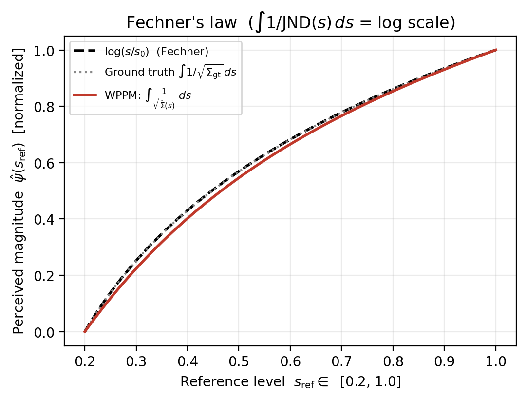
\[ \delta_\mathrm{th}(s) = k\,s \qquad\Longleftrightarrow\qquad \frac{\delta_\mathrm{th}(s)}{s} = k . \]

Heavier baselines need proportionally larger changes; the fraction $k$ stays fixed. Fechner's law is the corollary you get by walking the stimulus axis one JND at a time perceived magnitude grows logarithmically:

\[ \psi(s) = \int_{s_0}^{s}\frac{1}{\delta_\mathrm{th}(s')}\,\mathrm{d}s' = \frac{1}{k}\ln\frac{s}{s_0}. \]

The WPPM (Wishart Process Psychophysical Model) does not assume any of this. It learns a field of discrimination noise $\Sigma(s)$ over stimulus space and lets the law fall out of the data. So we can run a clean experiment:

Recovering Weber's Law predictions as a unit test for models of perception

Generate binary oddity responses from a synthetic observer that obeys Weber's law exactly. Hand the WPPM only those responses (never $k$ and the never the linear form). If it recovers a noise function whose implied threshold scales linearly with $s$, the model is flexible enough to represent Weber's law. WPPM-recovers-Weber becomes a 'unit test ' for the package.

Weber's law in WPPM language¶

The WPPM parametrizes a square root of the covariance, $\Sigma(s) = U(s)\,U(s)^\top$, which guarantees $\Sigma$ stays positive. In 1-D this is just $\sqrt{\Sigma(s)} = U(s)$, and $\sqrt{\Sigma(s)}$ is our JND proxy (threshold $\propto$ noise SD).

So Weber's law translates to a single line:

\[ \underbrace{\delta(s)}_{\text{JND}} = \underbrace{k\,s}_{\text{Weber}} = \underbrace{\sqrt{\Sigma(s)} = U(s)}_{\text{what the WPPM learns}} \;\;\Longrightarrow\;\; \Sigma(s) = (k\,s)^2 . \]

$U(s)$ is represented in a Chebyshev basis over a normalized coordinate $x\in[-1,1]$, $U(x)=\sum_i W_i\,T_i(x)$. Because Weber needs $U$ linear, a degree-1 basis ($U(x)=W_0+W_1 x$, two parameters) is exactly sufficient but we deliberately fit a more flexible model (degree 3 polynomial) and check it doesn't overfit.

Runtime¶

Hardware	Approximate time
CPU (laptop / M-series Mac)	1–3 min

The fit uses N_TRIALS = 2000 trials and MC_SAMPLES = 1000 Monte-Carlo draws per trial; the optional basis sweep at the end refits the model several times and is the slow part.

Step 1 Stimulus domain and coordinates¶

The Chebyshev basis we use requires stimuli to be in $[-1, 1]$. We pick a physical range [S_MIN, S_MAX] wide enough to hold the largest comparison and map physical $s$ to normalized $x$ explicitly:

Physical range and coordinate transforms
S_MIN: float = 0.2  # domain minimum (also minimum reference; must be > 0 for Weber)
S_MAX: float = 2.0  # domain maximum; wide enough to cover all comparisons,
# which are an offset from reference stimulus.
# worst-case: S_MAX_REF*(1 + max_jnd_multiples*K_WEBER) = 1.0*1.8 = 1.8 < 2.0.
S_MAX_REF: float = (
    1.0  # maximum reference stimulus; references sampled from [S_MIN, S_MAX_REF].
)


def to_norm(s: jnp.ndarray) -> jnp.ndarray:
    """Map physical s (anywhere in [S_MIN, S_MAX]=[0.2, 2.0]) -> normalized x in [-1, 1].
    The domain covers both references [S_MIN, S_MAX_REF] and comparisons up to S_MAX."""
    return 2.0 * (s - S_MIN) / (S_MAX - S_MIN) - 1.0


def to_phys(x: jnp.ndarray) -> jnp.ndarray:
    """Map normalized x in [-1, 1] -> physical s in [S_MIN, S_MAX] = [0.2, 2.0]."""
    return 0.5 * (x + 1.0) * (S_MAX - S_MIN) + S_MIN

References are drawn from [S_MIN, S_MAX_REF] = [0.2, 1.0]; comparisons can reach up to S_MAX_REF·(1 + 4·k) = 1.8, comfortably inside S_MAX = 2.0.

Step 2 The ground-truth Weber observer¶

This is the synthetic participant that generates our data. It implements only the one method OddityTask needs a square-root covariance U and hard-codes Weber's law, $\sqrt{\Sigma(s)} = k\,s$. It receives the same normalized $x$ as the WPPM and converts back to physical $s$ internally, so simulation and fitting share one coordinate system.

Step 3 Simulate oddity-task data¶

The experiment settings:

Settings
K_WEBER = 0.2  # Weber fraction (ground truth)
DIAG_TERM = 1e-6  # numerical stability jitter; shared by WeberGroundTruth AND the
# fitted WPPM so the generative model and the fitting model have
# identical parameterisations. Removing from WPPM risks NaN gradients
# when U(x) \approx 0 during early optimisation
N_TRIALS = 2000
MC_SAMPLES = 1000  # MC samples for simulation and fitting

# degree-1 U(x) = W_0 + W_1*x; sufficient for Weber (linear U -> quadratic Sigma).
# W shape (2, 1, 1) = 2 parameters with extra_dims=0. See module docstring.
BASIS_DEGREE = 1

NUM_STEPS = 500  # 1000 gets close for 3 param model (0 additional embedding dims)
LEARNING_RATE = 5e-4

Each trial is a 3-AFC oddity: two identical references and one comparison; the observer picks the odd one out. We place each comparison a random number of JNDs (0.5–4) above its reference, so the data spans easy and hard trials, then draw a binary correct/incorrect response from the Monte-Carlo oddity likelihood.

The stored TrialData holds only (stimuli, responses) exactly what an experimenter records. Plotting reference level $s$ against displacement $\delta = s_\mathrm{comp} - s_\mathrm{ref}$, with the ground-truth JND line $\delta = k\,s$, shows the structure the model must recover: trials above the line are mostly correct, below mostly wrong.

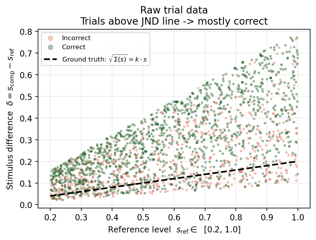
Raw trial scatter: correct (green) and incorrect (red) trials vs reference level and displacement, with the ground-truth JND line

The model sees only these binary outcomes never the dashed ground-truth line.

Step 4 Fit a 1-D WPPM¶

We build a WPPM with a degree-3 Chebyshev basis more flexibility than Weber needs and fit it by MAP. Crucially, the model sees only the responses: never $k$, never the linear form. (BASIS_DEGREE_FIT = 3 is set just above this block in the script.)

Build and fit with MAPOptimizer
prior = Prior(input_dim=1, basis_degree=BASIS_DEGREE_FIT, extra_embedding_dims=0)
model = WPPM(
    input_dim=1,
    extra_dims=0,  # embedding_dim = input_dim (minimal)
    prior=prior,
    likelihood=task,
    noise=GaussianNoise(sigma=0.0),
    diag_term=DIAG_TERM,  # matches WeberGroundTruth for a fair comparison
)

init_params = model.init_params(jr.PRNGKey(1))

optimizer = MAPOptimizer(
    steps=NUM_STEPS,
    learning_rate=LEARNING_RATE,
    track_history=True,
    log_every=1,
)

map_posterior = optimizer.fit(model, data, init_params=init_params, seed=2)

MAPOptimizer runs SGD + momentum and returns a posterior whose .params are the fitted Chebyshev weights $W$.

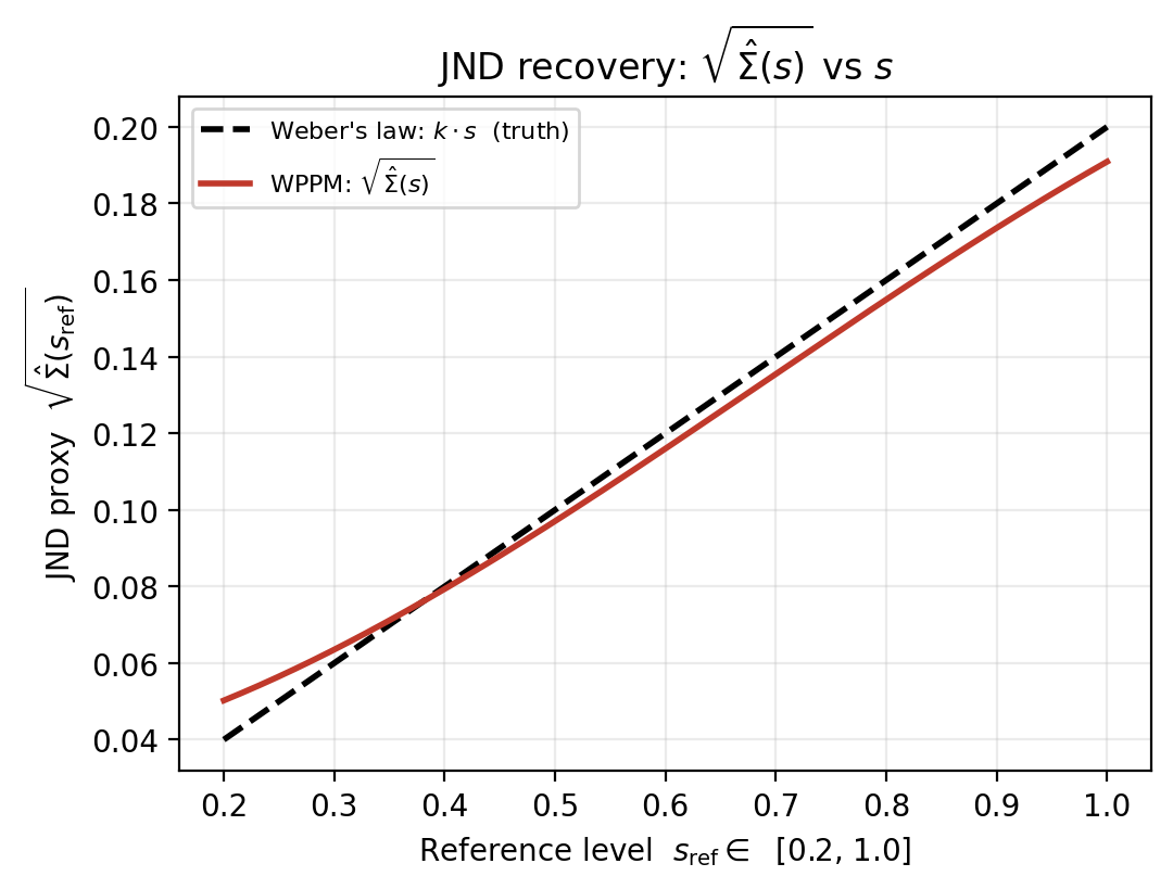
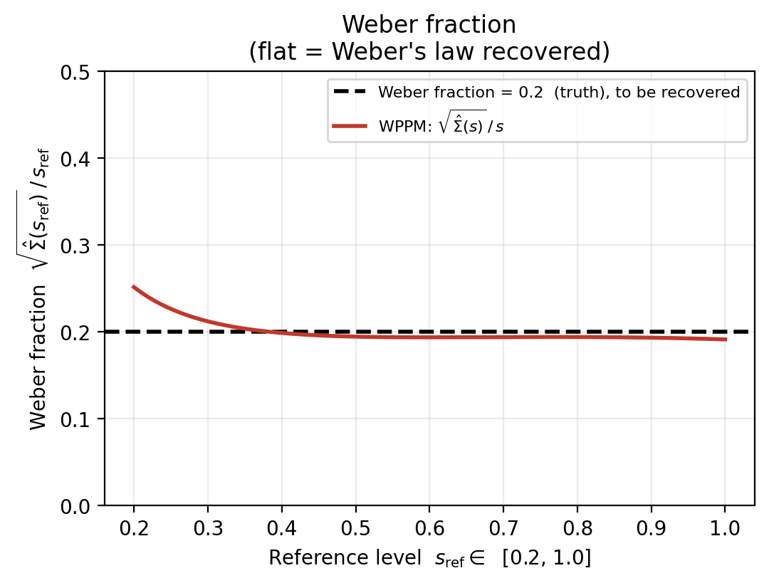
Step 5 Read the recovered function three ways¶

Bind the fitted parameters into a WPPMCovarianceField and evaluate $\Sigma(s)$ on a dense grid. From the single fitted function $\sqrt{\hat\Sigma(s)}$ we read three views the first three panels are the same fit re-expressed.

Derived quantities: JND and Weber fraction
# Dense grid over the reference range for analysis and plotting.
# Comparisons may extend above S_MAX_REF, but we only evaluate the sub-range
# [S_MIN, S_MAX_REF] where the model is well-determined by training data.
s_grid = jnp.linspace(S_MIN, S_MAX_REF, 300)  # physical, reference range
x_grid = to_norm(s_grid)[:, None]  # normalized, shape (300, 1)

# Bind fitted parameters to the model: creates a callable x -> Sigma(x).
fitted_cov_fn = WPPMCovarianceField(model, map_posterior.params)
variances = fitted_cov_fn(x_grid)  # (300, 1, 1); 1x1 "matrix" per grid point;
# [:, 0, 0] extracts the scalar Sigma(s)
# sqrt(Sigma) from WPPM; proxy for implied JND in physical units
# (valid in the 1D equal-variance limit; see module docstring)
jnd_fitted = jnp.sqrt(variances[:, 0, 0])
jnd_truth = K_WEBER * s_grid  # ground truth: k*s

# Weber fraction: JND(s)/s; should be flat at K_WEBER
weber_fraction_fitted = jnd_fitted / s_grid

(a) JND recovery. $\sqrt{\hat\Sigma(s)}$ vs $s$ should be a straight line through the origin with slope $k$.

Recovered JND proxy sqrt(Sigma_hat) vs s, overlaid on the Weber ground truth k*s

(b) Weber fraction Divide by $s$: $\sqrt{\hat\Sigma(s)}/s$ should be flat at $k = 0.2$. A flat line is the defining signature of Weber's law in this figure.

$Weber fraction sqrt(Sigma_hat)/s vs s, flat at 0.2$

(c) Fechner's law for free. Integrate $1/\sqrt{\hat\Sigma(s)}$; the result is the logarithmic sensation scale a deterministic transform of the same curve the model was never fit to.

Fechner sensation curve: integral of 1/JND follows log(s)

Step 6 Behavioral check: psychometric curves¶

The three views above are algebra are '3 sides of the same coin'.

Psychometric curve:¶

For 3 stimulus reference levels we sweep the comparison and predict $p(\text{correct})$ from the fitted model (and from the ground truth, for comparison):

If Weber's law has been recovered, the sigmoids shift right in proportion to $s$: a larger baseline needs a proportionally larger $\delta$ for the same performance. Chance for a 3-AFC oddity task is $1/3$.

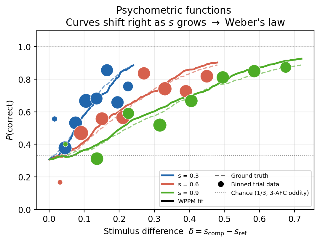
Psychometric curves for three reference levels, shifting right with s; WPPM fit vs ground truth with binned data

Solid: WPPM fit. Dashed: ground truth. Dots: binned trial data that the model was fitted on overlayed for reference. Larger dots mean more data in that vicinity. The model inputs .

Step 7 Learning curve and the full picture¶

The optimizer's history is the negative log-posterior per step:

Access the learning curve
steps_hist, loss_hist = optimizer.get_history()  # (step indices, neg-log-posterior)

The script assembles every result (the four diagnostic panels, the psychometric curves, and this learning curve) into one figure:

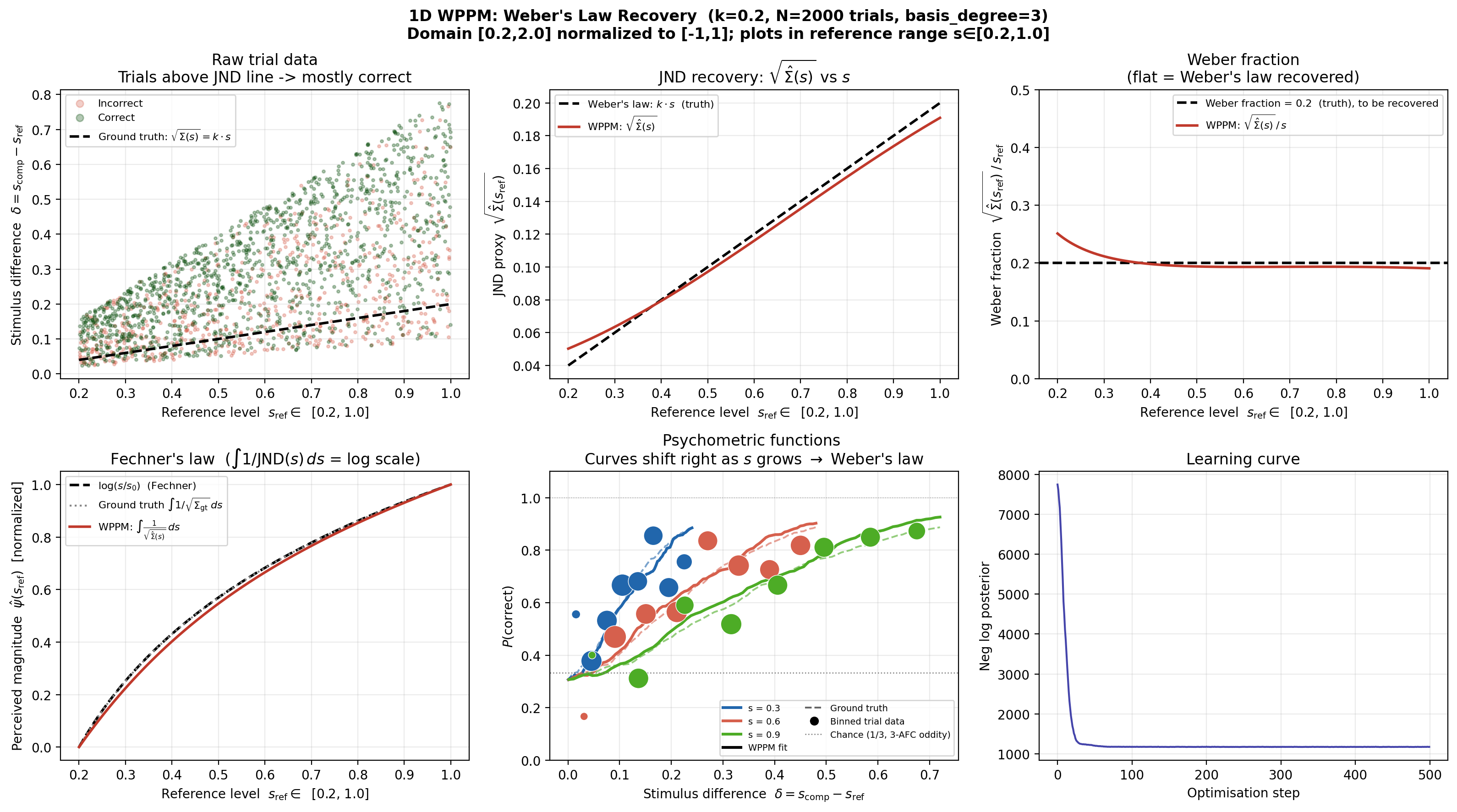
$Combined six-panel figure: trial scatter, JND recovery, Weber fraction, Fechner, psychometric curves, and learning curve$

All results at a glance; the learning curve is the bottom-right panel.

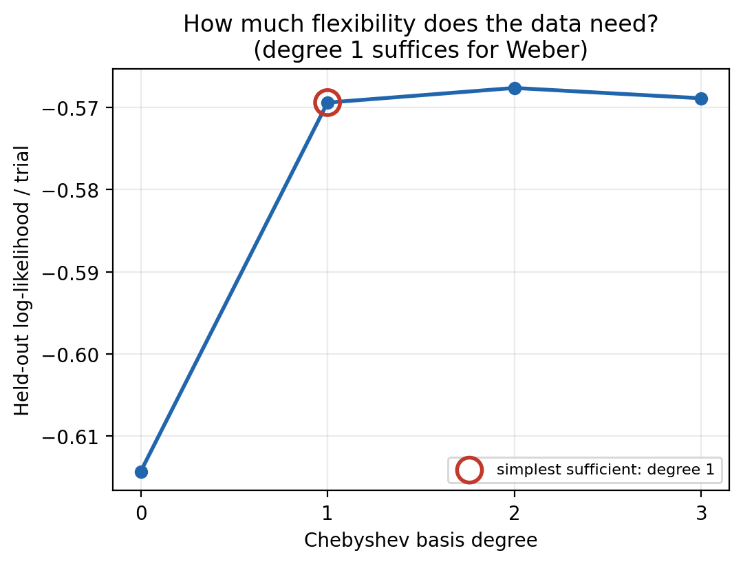
Step 8 How much flexibility did the data actually need?¶

We fit a degree-3 model, but Weber only needs degree 1. Training fit alone can't tell us which is right (more parameters never fit worse), so we split the trials, fit on the training set across several basis degrees, and score the held-out log-likelihood:

Degree 0 (a constant $U$, hence a constant JND) cannot bend and underfits; degree 1 (linear $U$ -> quadratic $\Sigma$) peaks; degree 2+ adds no held-out gain. The data needs exactly the flexibility Weber's law implies, ie, linear.

Held-out log-likelihood per trial vs Chebyshev basis degree; degree 1 is the simplest sufficient model

Verdict

Given only binary "which is different?" answers, the WPPM with no linear law encoded recovers everything Weber's law predicts: a constant fraction, a logarithmic sensation scale, and psychometric curves that shift with stimulus level. The unit test passes :)

Next steps¶

Your own data: replace the simulated TrialData with real stimuli and responses, and validate via held-out psychometric curves where no ground truth exists.
Beyond Weber: the same machinery represents other regimes (e.g. de Vries–Rose $\delta_\mathrm{th}\propto\sqrt{s}$) -> fit them the same way and read off the recovered law.
Fewer trials: put trials where uncertainty is highest with adaptive trial placement.
API reference: MAPOptimizer, WPPM, and WPPMCovarianceField.
2-D workflow: the quick start and the full WPPM example fit spatially-varying covariance ellipses.