Plotting covariance ellipse fields¶

A 2×2 covariance drawn as an ellipse is how psyphy shows most of what it computes: a model's internal noise field, a threshold contour, a posterior draw. psyphy.viz.plot_ellipses draws any of those, one field or several.

pip install 'psyphy[viz]'     # matplotlib is an optional dependency

Import
from psyphy.viz import plot_ellipses  # noqa: E402

Runnable script: ellipse_plots.py. Everything below is synthetic and runs in about a second.

The example field
def example_field(n_side: int = 5) -> tuple[np.ndarray, np.ndarray]:
    """A grid of reference points and one 2x2 covariance at each.

    Ellipses grow with distance from the origin and are oriented radially --
    loosely the structure seen in color-discrimination data.
    """
    axis = np.linspace(-0.7, 0.7, n_side)
    centers = np.stack(np.meshgrid(axis, axis), axis=-1).reshape(-1, 2)

    radius = np.linalg.norm(centers, axis=1)
    angle = np.arctan2(centers[:, 1], centers[:, 0])
    covs = np.empty((len(centers), 2, 2))
    for i, (r, a) in enumerate(zip(radius, angle, strict=True)):
        lengths = np.diag([(0.02 + 0.05 * r) ** 2, (0.02 + 0.015 * r) ** 2])
        rot = np.array([[np.cos(a), -np.sin(a)], [np.sin(a), np.cos(a)]])
        covs[i] = rot @ lengths @ rot.T
    return centers, covs

One field¶

Pass centers and one (n_points, 2, 2) stack. The default scale=1.0 draws true size: the ellipse semi-axes are the square roots of the covariance eigenvalues, in the units of your stimulus space.

centers, covs = example_field()

# One field. The default scale=1.0 draws true size. ellipses are small
# relative to the grid.
fig, ax = plt.subplots(figsize=(5, 5), dpi=150)
plot_ellipses(centers, covs, ax=ax, colors="C0", show_centers=True)

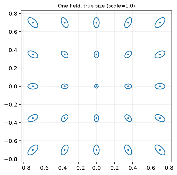
Nothing is saved or shown for you. Instead, the function draws into an Axes and returns it, so the figure stays yours to title, style, and save.

Several fields overlaid¶

Pass a list of fields to compare them. This is the "published vs. fitted" figure that shows up throughout the WPPM examples.

# Two fields overlaid. scale="auto" sizes them to the grid, and returns the
# factor so the figure can report it. Both fields share that one factor --
# otherwise their relative sizes would be meaningless.
inflated = covs * 1.6**2  # 1.6x larger radii
fig, ax = plt.subplots(figsize=(5, 5), dpi=150)
ax, scale = plot_ellipses(
    centers,
    [covs, inflated],
    ax=ax,
    scale="auto",
    colors=["black", "crimson"],
    linestyles=["--", "solid"],
    labels=["reference", "comparison"],
    return_scale=True,
)

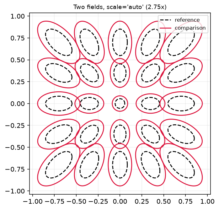
colors, linestyles, linewidths, alpha, and labels each accept either one value for all fields or a list with one entry per field. A legend appears only if you pass labels.

scale='auto' sizes ellipses to the grid and shares one factor

True size is honest but can be hard to read: on a dense grid the ellipses shrink to specks, and on a coarse one they float in white space. scale="auto" sets the median ellipse to a fixed fraction of the median spacing between centers, so the same call works on a 7×7 grid and a 103×103 one.

Two things follow. It is not always a magnification: on a dense grid the factor drops below 1, shrinking ellipses so they do not overlap. And when several fields are drawn, the factor is computed from the first one and applied to all of them; independently scaled fields could not be compared by eye. Pass return_scale=True to get the number back and put it in your title, since a rescaled figure cannot be read for absolute size.

Posterior draws¶

A (n_samples, n_points, 2, 2) array draws one translucent field per sample; the natural way to show parameter uncertainty.

# A (n_samples, n_points, 2, 2) stack draws one translucent field per
# sample. This is what posterior draws would look like.
samples = covs[None] * RNG.normal(1.0, 0.12, size=(12, len(centers), 1, 1)) ** 2
fig, ax = plt.subplots(figsize=(5, 5), dpi=150)
plot_ellipses(centers, samples, ax=ax, scale="auto", colors="C3", alpha=0.25)

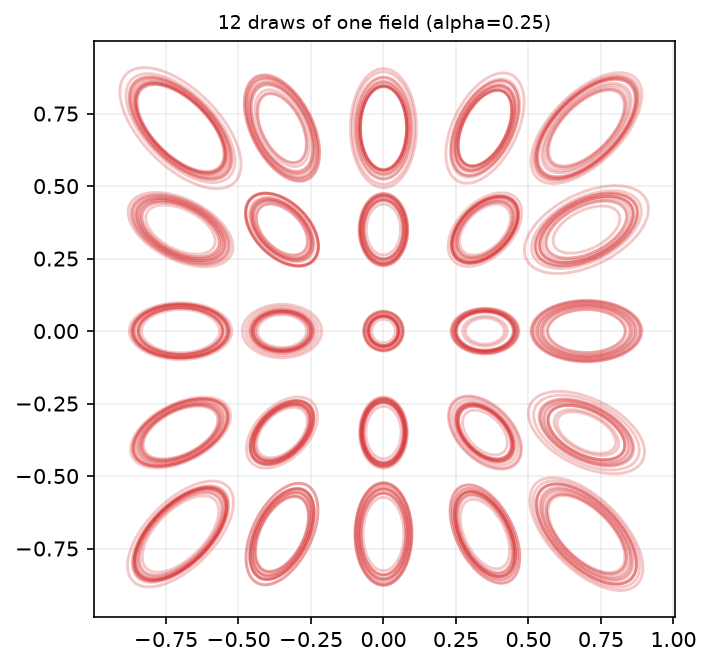
This is the shape WPPMPredictivePosterior.rsample() returns. With a MAPPosterior every draw is identical (a point estimate has no spread), so the band collapses to a single field.

Per-ellipse colors¶

colors also accepts an (n_points, 3) or (n_points, 4) array, giving each ellipse its own color. That is how the Hong et al. reproduction colors each contour by its own reference stimulus:

colors = hong2025.w2d_to_rgb(coords, M)          # (n_points, 3)
plot_ellipses(coords, thresholds, colors=colors)

Non-positive-definite covariances¶

A covariance that is not positive-definite has no ellipse. By default those are skipped and a warning names how many were dropped:

1 2	`UserWarning: 3 non-positive-definite covariance(s) were not drawn; the plotted field is incomplete.`

Silence is the wrong default here, a field quietly missing a few ellipses is hard to spot by eye, and it usually means something upstream went wrong, such as an ill-conditioned threshold inversion. Pass skip_non_pd=False to raise instead.

Without matplotlib¶

The geometry is separate from the drawing, in psyphy.viz.geometry, and needs only numpy and scipy. Use it to feed another plotting backend, or to test without a display:

from psyphy.viz import ellipse_segments

segments, valid = ellipse_segments(centers, covs, scale=1.0)
# segments: list of (n_points, 2) arrays, one per positive-definite covariance
# valid:    bool mask of which covariances were drawable

Limits¶

2-D only. Higher-dimensional covariances raise NotImplementedError; drawing them would mean ellipsoid rendering.
scale="auto" needs at least two centers, since it measures spacing between them. With one point, pass an explicit scale.