Reproducing Hong et al. (2025)

This tutorial is accompanied by a runnable script: hong2025_reproduction.py.

How to run the script

An install of psyphy on its own is not enough: the figures here need a plotting backend, which psyphy does not depend on.

pip install 'psyphy[viz]'     # psyphy + matplotlib, all this page needs
pip install 'psyphy[cuda]'    # also, for the refit: JAX's CUDA build

viz is matplotlib and nothing else. (There is also a broader examples extra that adds seaborn and JupyterLab for the other pages; this one does not need it.) The refit at the paper's settings wants an NVIDIA GPU . Everything else on this page runs on a laptop.

Everything on this page comes from one script. Pick a mode by how much compute you want to spend:

# stages 1 and 2 only: the exact check and Figure 2B. <1 min on CPU.
python hong2025_reproduction.py --skip-refit

# add stage 3, the refit at the paper's settings. Wants a GPU.
python hong2025_reproduction.py --mode full

To check the code path runs on your laptop before committing to any of that:

# a smoke test, not a reproduction: 500 trials and 20 steps
# leave the fit essentially at its prior.
python hong2025_reproduction.py --mode quick

Can psyphy reproduce a published result, starting from the raw data? This page answers that for Hong et al. (2025): refit the model from their trials, invert it to discrimination thresholds, and compare against the figure they published. The answer is yes: our threshold contours fall inside the authors' own 95% bootstrap interval at all of their 49 reference points.

Disclaimer: Their experiment was about color, so this page is too; but the model and psyphy's implmentation generalize! See Scope below.

How this tutorial is laid out First, we introduce the task and show the headline result: the paper's Figure 2B, reproduced. Then we cover the practical parts, e.g., loading the published data, and building paper's model. The reproduction itself is then built up one question at a time, so that a disagreement at any point tells us where it came from:

1. Given the published weights, do we compute the same covariance field?
2. Given the published weights, do we recover the same threshold contours (Figure 2B)?
3. Given only the raw trials, do we refit the same weights?
4. Putting 2 and 3 together: from raw trials alone, do we reproduce the same published figure 2B?
5. And is that agreement good enough, measured against the paper's own bootstrap confidence interval?

That order is backwards on purpose. Questions 1 and 2 hand psyphy the paper's own weights, so the expensive optimization doesn't run. If they fail, the bug is in our model code. Question 3 is the first that fits anything, and fitting is both the slow part and the part with the most ways to go wrong. Checking the cheap, deterministic parts first means that if question 3 disagrees, the optimizer is the only suspect left.

Who this is for

• You want a worked example of psyphy on real data, with an external ground truth to check against.
• You know the paper and want to see how psyphy reproduces it.

No familiarity with the model is needed to start. The next section introduces it at a high level. See the paper itself for the full reference:

Hong, F., Bouhassira, R., Chow, J., Sanders, C., Shvartsman, M., Guan, P., Williams, A. H., & Brainard, D. H. (2025). Comprehensive characterization of human color discrimination thresholds. eLife 14:RP108943. https://doi.org/10.7554/eLife.108943.2

---

Background — what the Whishart Psychophysical Process Model (WPPM) is

Measuring a discrimination threshold the usual way means fixing one color and asking, over many trials, how far a second color has to move before someone notices the difference. That tells you about one color. Repeating it across a whole plane of colors is impractical: too many locations and far too many trials, so we run into the curse of dimensionality.

The WPPM takes a different approach. It assumes the observer's internal noise changes smoothly across color space: nearby colors are confusable in similar ways. That lets us fit one smooth field over the entire space instead of many separate measurements, so every trial informs the whole picture. Once fit, we can evaluate the model at any point in stimulus space, including those we haven't tested!

psyphy implements the Wishart Psychophysical Process Model (WPPM) in general form: any number of stimulus dimensions, any task you can write a likelihood for. The color setup here is only one configuration of it, which is why this page doubles as an external check on psyphy and a worked example of the general pipeline. The WPPM approach carries beyond color to any domain where the noise limiting performance varies smoothly across the stimulus space.

Hong et al. collect each judgement from the human subjects with an oddity task: on every trial the observer sees three stimuli (two identical, one different) and picks the odd one out. Chance is therefore 1/3, and the threshold is placed at the usual midpoint between chance and perfect performance, P(correct) = 2/3. That is the 66.7% contour this page reproduces.

---

Scope

For this tutorial we will describe the WPPM in terms of color, because that is what Hong et al. measured. The WPPM itself is not specific to color: it models noise varying smoothly over any stimulus space, for any task you can write a likelihood for. See Recovering Weber's Law for a one-dimensional example, or the simulated-data walkthrough.

The result

Each ellipse is a Just-Noticeable Difference (JND) threshold contour around a reference color at its center: the smallest color difference this observer can reliably detect. Operationally, it is how far a comparison color must move from the reference before they pick it out as the odd one 66.7% of the time. It is an ellipse rather than a circle because sensitivity depends on direction; some color changes are easier to see than others of the same magnitude. The orientation and elongation of each ellipse are exactly what the WPPM estimates. We can also see that the sizes of the ellipses increase as you move away from the origin in the plot below, which corresponds to a gray stimulus. This is a reproduction of the Weber–Fechner law.

See Recovering Weber's Law for a worked example reproducing the classic Weber's Law result on simulated one-dimensional data.

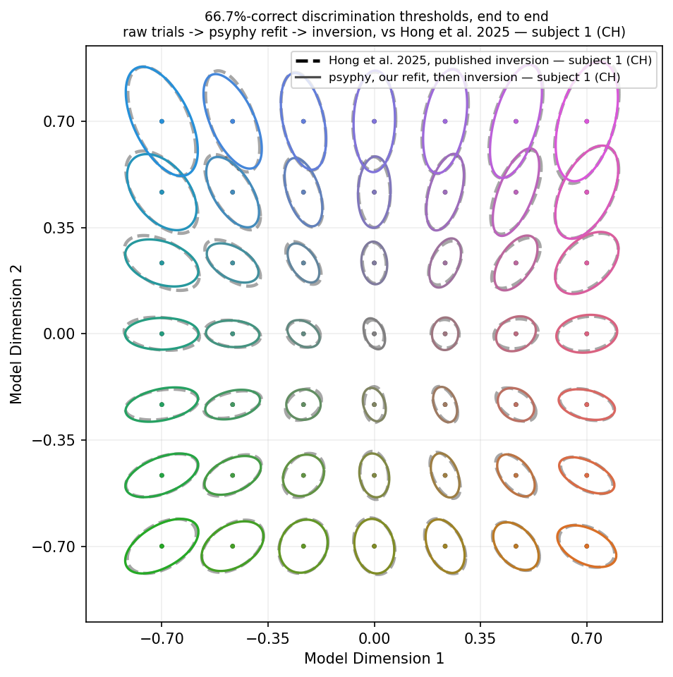
Paper Figure 2B, reproduced end to end for subject 1 (CH). Colored ellipses are the contours psyphy recovers; dashed gray are the published ones. Each ellipse takes the color of its own reference stimulus (center dot). Nothing published enters this chain except the raw trials: psyphy fits the model's weights from those trials, and inverts the oddity task to turn the resulting noise field into 66.7%-correct thresholds (represented as ellipses). The axes are model dimensions, which arbitrary up to an affine transformation of the input (RGB) space.

The whole recipe

The block below is the short version: download one observer's data, load the paper's fitted weights, and turn them into threshold contours. It runs as it stands, on a laptop. The sections after it go through the same steps slowly, and add the refit that produces the figure at the top of this page, and reproduce the fit from scratch with psyphy's implementation.

import jax

jax.config.update("jax_enable_x64", True)  # the authors used float64

import jax.numpy as jnp  # noqa: E402

from psyphy.data.published import hong2025  # noqa: E402
from psyphy.posterior import (  # noqa: E402
    MAPPosterior,
    ThresholdConfig,
    WPPMPredictivePosterior,
)

paths = hong2025.fetch(subject=1)  # download from OSF
W = hong2025.load_reference_W(paths["weights"])  # the paper's fitted weights
# W = jnp.asarray(np.load("fits/hong2025_full_fit.npz")["W"]) # for full refit
coords, published = hong2025.load_sigma_table(paths["thres_ellipses"])

# Model: given weights W, how noisy is perception at each color?
model = hong2025.build_paper_model(mc_samples=2000)

# Parameter posterior: which W do we believe?
posterior = MAPPosterior({"W": W}, model)

# Search settings: how carefully to look for each threshold
# These are the paper's own: 16 directions, 1000 distances along each
config = ThresholdConfig(n_theta=16, n_length=1000)

# Predictive posterior: given what we believe about W, what do we predict here?
thresholds = WPPMPredictivePosterior(
    posterior,
    jnp.asarray(coords),  # reference points only
    n_samples=1,
    threshold_pred=True,  # ask for thresholds
    threshold_config=config,
).mean  # -> (49, 2, 2)

# This used the authors' weights, so it reproduces their published inversion
# rather than the figure at the top of the page. To go end to end instead, fit
# your own weights (see Refit) and change only where W comes from:
#
#   W = jnp.asarray(np.load("fits/hong2025_full_fit.npz")["W"])
#
# The model, the config and the call above are identical either way.

---

Data

Psyphy makes it easy to download the published data:

paths = hong2025.fetch(subject=args.subject, noise_ellipses=args.noise_ellipses)

What each data file is, and how big

File	Size	Used for
trial_data_pooled_by_type_sub1.csv	1 MB	trials, for the refit
Bestfit_W_sub1.csv	212 KB	fitted weights, plus 120 bootstraps
Thres_ellipses_sub1.csv	320 KB	the 7x7 grid and published thresholds
Noise_ellipses_sub1.csv	68 MB	published \(\Sigma_{\text{noise}}\) on a 103x103 grid

load_trials loads in the published file and returns psyphy's TrialData object, so it will work directly with our methods:

# Only the AEPsych trials were used for the published fit; the MOCS trials
# in the same file are held-out validation. This is the default.
data = hong2025.load_trials(
    paths["trials"], max_trials=cfg["max_trials"], seed=seed
)

The published data holds 12,000 trials in two equal halves: 6,000 AEPsych_* rows (5,100 adaptive placement plus 900 Sobol) used for fitting, and 6,000 MOCS_* rows held out for validation. For this tutorial and the figures, we only use the rows used for fitting (by default load_trials loads only the rows used for fitting). Pass trial_types=("MOCS",) for the held-out half, or trial_types=None for all 12,000.

Fitting all 12,000 trials does not reproduce the paper

It gives a plausible result that is not the published one.

For more information on how the authors did adaptive trial placement using the library AEPsych, we refer the reader to the paper.

Two conventions worth knowing when you inspect the loaded data

psyphy stores trials as a stimuli array of shape (N, K, d) — trials x stimuli per trial x stimulus dimensions — alongside responses; see TrialData.

Oddity trials are stored with K=2, not 3. Each trial shows three stimuli (reference, reference, comparison)but only two distinct ones, and K counts distinct stimuli. So data.stimuli comes back (6000, 2, 2) for a three-interval task. The repetition is applied inside the oddity likelihood rather than stored on every row.

---

Model

build_paper_model() assembles a WPPM from the settings the paper used, which we transcribed once into PAPER_HYPERPARAMS.

The paper's hyperparameters in full

Grouped by what each one controls.

PAPER_HYPERPARAMS: Mapping[str, Any] = {
    # -- Covariance field: what shapes the noise field can take ------------
    # Highest Chebyshev degree, i.e. T0..T4 per input dimension -> a 5x5
    # coefficient grid. The paper writes this as degree=5, counting basis
    # *functions* rather than degrees. Same model, different convention.
    "basis_degree": 4,
    # Stimulus dimensionality: the 2-D isoluminant chromatic plane.
    "input_dim": 2,
    # Extra embedding dimensions for U(x), where Sigma = U U^T + diag_term * I
    # and U has shape (input_dim, input_dim + extra_dims). The extra column
    # lets Sigma stay full rank instead of being a bare rank-2 outer product.
    "extra_dims": 1,
    # -- Prior over the basis weights W ----------------------------------
    # Prior variance of a degree-0 coefficient: the overall scale of the noise
    # field before any data is seen.
    "variance_scale": 3e-4,
    # A degree-d coefficient has prior variance variance_scale * decay_rate^d,
    # so higher-frequency terms are shrunk harder. Smaller -> smoother field.
    "decay_rate": 0.4,
    # The delta added to Sigma's diagonal. psyphy's default is 1e-6,
    # which is safer for numerical stability.
    "diag_term": 0.0,
    # -- Oddity likelihood: how P(correct) is estimated --------------------
    # Monte Carlo draws per trial. P(correct) has no closed form, so it is
    # estimated by sampling; this dominates the cost of a fit.
    "mc_samples": 2000,
    # Width of the logistic that smooths the hard "is the odd one furthest?"
    # comparison, so the MC estimate stays differentiable for gradient descent
    "bandwidth": 5e-3,
    # -- MAP optimizer, used by the refit only -----------------------------
    "learning_rate": 1e-4,  # gradient step size
    "momentum": 0.2,  # 'heavy-ball' momentum
    "total_steps": 1500,  # gradient steps per restart
    "n_restarts": 1,  # independent prior draws; the lowest final loss wins
    # Hong et al tried 3, but 1 is enough to reproduce the published fit.
    # -- Reporting ---------------------------------------------------------
    # The criterion the paper's thresholds are defined at: midway between
    # chance (1/3) and perfect, for a 3-alternative task
    "target_pC": 0.667,
}

---

Exact check

does psyphy build the same covariance field Hong et al published?

With the data loaded and the model built, we start with the question that has no moving parts. Hand psyphy the paper's own weights and ask it for the covariance field: no optimizer and nothing random. If this disagrees, the problem is in the model implementation itself, and everything downstream would be built on sand.

W_org = hong2025.load_reference_W(paths["weights"])  # (5, 5, 2, 3)
coords, sigma_published = hong2025.load_sigma_table(paths["noise_ellipses"])

model = hong2025.build_paper_model(mc_samples=1)  # MC unused: no likelihood here
field = WPPMCovarianceField(model, {"W": W_org})
sigma_psyphy = np.asarray(field(jnp.asarray(coords)))

max_abs = float(np.abs(sigma_psyphy - sigma_published).max())

In the above, we're simply computing the difference between our computed covariances and the values shared by the paper's authors, for all 42,436 ellipses. The maximum value of the differences are shown below:

max |diff|   : 6.778e-09
mean |diff|  : 2.538e-09

Our values agree to all published didgits in 96% of the cases and, in the final 4%, only differ by +/- 1 in the last printed digit. This is agreement to the precision the file can express.

This runs as a test (test_covariance_field_matches_published_sigma_noise), skipped automatically when the data has not been downloaded, so CI stays network-free.

---

That settles the model implementation: given the same weights, psyphy builds the same field. The next question is whether we can turn that field into the thresholds the paper actually reports.

Thresholds (as in Paper Figure 2B)

The model is parameterized in \(\Sigma_{\text{noise}}(x)\), the covariance of the observer's internal representation. The paper reports thresholds, i.e., how much do we have to move in stimulus space, until the observer picks it out as the odd one 66.7% of the time. Those are different objects! The map between them runs in two directions, and only the forward pass is easy:

• Forward: given the noise at two points, how often does the observer get the trial right? That is what the model computes directly.
• Inverse: given that they get it right two-thirds of the time, how far apart were the stimuli? That is what Figure 2B plots and it is the direction with no closed form.

Written out:

\[ \begin{aligned} \text{forward (psyphy's OddityTask)}:\qquad & \Sigma_{\text{noise}}(x_{\text{ref}}),\ \Sigma_{\text{noise}}(x_{1}) && \longrightarrow\ P(\text{correct}) \\[4pt] \text{inverse (what Figure 2B plots)}:\qquad & P(\text{correct}) = \tfrac{2}{3} && \longrightarrow\ x_{1} \end{aligned} \]

There is no closed form for the inverse. For the 3-alternative oddity task the observer is correct when the two identical stimuli are nearer to each other than either is to the odd one:

\[ P(\text{correct}) \;=\; \Pr\!\left[\min(d_{02},\, d_{12}) > d_{01}\right] \]

where \(d_{ij}\) is the Mahalanobis distance between the internal representations of stimuli \(i\) and \(j\). This is the distance that measures separation in units of the noise itself, so a step counts as large only relative to how noisy the representation is in that direction. That probability has no analytic form, which is why the paper estimates it by Monte Carlo in the first place. So we have to compute the inverse numerically following the procedure given in the paper:

1. Probe n_theta directions around each reference point.
2. Along each, evaluate P(correct) at n_length distances and keep the one closest to 2/3. We thus have one boundary point per direction.
3. Fit an ellipse to those n_theta points. This step does have a closed-form solution and so can be done quickly.

Step 3 needs no optimizer, the ellipse fit is closed-form.

To compute this inverse using psyphy, we construct the WPPMPredictivePosterior object with the threshold_pred argument set to True, passing it the relevant arguments.

Why the ellipse fit is closed-form

A point at radius r in direction u satisfies \(u^TΣ^{-1}u = 1/r^2\), which is linear in the three free entries of \(Σ^{-1}\). So the fit is least squares over those three unknowns, followed by a single matrix inverse to recover \(Σ\) itself. No iteration, and nothing that can fail to converge.

We run the inversion at the paper's own settings (16 directions, 1,000 distances along each, 2,000 Monte Carlo samples per evaluation). That costs about 11 minutes on CPU for the 49 reference points.

Threshold settings

THRESHOLD_SETTINGS = {
    "paper": {
        "mc_samples": 2000,
        "config": ThresholdConfig(n_theta=16, n_length=1000),
    },
    "fast": {
        "mc_samples": 500,
        "config": ThresholdConfig(n_theta=16, n_length=300),
    },
}


# ---------------------------------------------------------------------------
# Comparison metrics
# ---------------------------------------------------------------------------
def _sqrtm_psd(M: np.ndarray) -> np.ndarray:
    """Matrix square root of a symmetric PSD matrix."""
    vals, vecs = np.linalg.eigh(M)
    return vecs @ np.diag(np.sqrt(np.clip(vals, 0.0, None))) @ vecs.T


def normalized_bures_similarity(A: np.ndarray, B: np.ndarray) -> float:
    """Normalized Bures Similarity between two PD matrices (1.0 == identical).

    The similarity measure Hong et al. use to rank bootstrap fits, reproduced
    here so the numbers are directly comparable to the paper's.
    """
    sa = _sqrtm_psd(A)
    inner = _sqrtm_psd(sa @ B @ sa)
    return float(np.trace(inner) / np.sqrt(np.trace(A) * np.trace(B)))


def compare_fields(Sigma_fit: np.ndarray, Sigma_ref: np.ndarray) -> dict[str, float]:
    """Compare two stacks of 2x2 covariances, shape (M, 2, 2).

    Compares Sigma  (never W ). U -> U Q for orthogonal Q leaves Sigma = U U^T
    unchanged and the prior is isotropic in the embedding axis, so the weights
    are not identifiable while the covariance field is.
    """
    rel_frob = np.linalg.norm(Sigma_fit - Sigma_ref, axis=(1, 2)) / np.linalg.norm(
        Sigma_ref, axis=(1, 2)
    )
    # Ellipse area is proportional to sqrt(det Sigma).
    area_ratio = np.sqrt(np.linalg.det(Sigma_fit) / np.linalg.det(Sigma_ref))

    def major_axis_angle(S: np.ndarray) -> np.ndarray:
        vecs = np.linalg.eigh(S)[1][..., -1]  # eigh returns ascending eigenvalues
        return np.arctan2(vecs[..., 1], vecs[..., 0])

    # Ellipse axes are undirected, so angle error lives on [0, 90] degrees.
    d_ang = np.degrees(major_axis_angle(Sigma_fit) - major_axis_angle(Sigma_ref))
    d_ang = np.abs((d_ang + 90.0) % 180.0 - 90.0)

    nbs = np.array(
        [
            normalized_bures_similarity(a, b)
            for a, b in zip(Sigma_ref, Sigma_fit, strict=True)
        ]
    )
    return {
        "rel_frobenius_median": float(np.median(rel_frob)),
        "rel_frobenius_max": float(rel_frob.max()),
        "area_ratio_median": float(np.median(area_ratio)),
        "angle_err_deg_median": float(np.median(d_ang)),
        "nbs_median": float(np.median(nbs)),
        "nbs_min": float(nbs.min()),
    }




# ---------------------------------------------------------------------------
# Plotting
#
# One convention across every comparison figure on this page, so the reader
# learns the legend once: the PUBLISHED field is black dashed at low alpha
# (reads as gray) and sits underneath; OURS is solid on top, colored by the
# reference stimulus via the monitor calibration matrix. Stages 2, 3, 4 and 5
# all follow it. The styling is spelled out at each call site rather than
# hidden behind a helper, because one of those calls is quoted in the docs.
# ---------------------------------------------------------------------------
# Every figure names its observer in the legend, on both curves, so a panel
# lifted out of the page cannot be mistaken for a different subject or for a
# group average. The paper fits each of its 8 observers separately; nothing
# here is ever pooled across them.
def _subject_tag(subject: int) -> str:
    """e.g. "subject 1 (CH)"."""
    return f"subject {subject} ({hong2025.SUBJECT_INITIALS.get(subject, '?')})"


def _published_label(subject: int, what: str = "published inversion") -> str:
    """Label for the authors' curve.

    ``what`` matters, because the figures do not all compare against the same
    published object. The threshold figures plot the authors' *published
    threshold table* -- contours they obtained by inverting their own fit -- so
    "published inversion" is the like-for-like counterpart to our inversion.
    The Sigma_noise figure plots no published table at all: it is psyphy's
    covariance field evaluated at their published weights, so it is labelled as
    weights rather than as a fit or an inversion.
    """
    return f"Hong et al. 2025, {what} — {_subject_tag(subject)}"


def _ours_label(subject: int, what: str) -> str:
    return f"psyphy, {what} — {_subject_tag(subject)}"


def _stimulus_colors(coords, M):
    """Per-reference RGB from the monitor calibration, or flat gray with a note.

    Returning the note rather than silently falling back means a gray figure
    cannot be mistaken for a correctly colored one.
    """
    if M is not None:
        return hong2025.w2d_to_rgb(coords, M), ""
    return (
        np.full((len(coords), 3), 0.45),
        "\nneutral gray \u2014 calibration matrix not downloaded",
    )


def _load_calibration():
    """Monitor calibration matrix, or None if it cannot be fetched."""
    try:
        return hong2025.load_calibration_matrix(hong2025.fetch_calibration_matrix())
    except Exception as exc:  # network, or OSF layout change
        print(f"  color calibration unavailable ({exc}); plotting in grey")
        return None


def plot_comparison(coords, Sigma_fit, Sigma_ref, out_path, title, scale, subject=1):
    """Two noise fields overlaid, published vs fitted.

    Published dashed gray underneath, as everywhere else on the page. Ours is a
    single red, *not* colored by reference stimulus: this is the noise field
    (the paper's supplementary Figure S3), and per-stimulus coloring is reserved
    for the threshold figures so the two cannot be mistaken for each other.
    """
    fig, ax = plt.subplots(figsize=(6, 6), dpi=150)
    plot_ellipses(
        coords,
        [Sigma_ref, Sigma_fit],
        ax=ax,
        scale=scale,
        colors=["black", "crimson"],
        linestyles=["--", "solid"],
        linewidths=[2.2, 1.6],
        alpha=[0.35, None],
        labels=[
            # Not "published Sigma_noise": this curve is psyphy's covariance
            # field evaluated at their published weights. Stage 1 shows the two
            # agree to 7e-9, but the curve on screen is ours, from their W.
            f"{_published_label(subject, 'published weights')}, \u03a3_noise",
            f"{_ours_label(subject, 'our MAP refit')}, \u03a3_noise",
        ],
        show_centers=True,
    )
    ticks = np.linspace(-0.7, 0.7, 5)
    ax.set_xticks(ticks)
    ax.set_yticks(ticks)
    ax.set_xlim(-1.0, 1.0)
    ax.set_ylim(-1.0, 1.0)
    ax.set_xlabel("Model Dimension 1")
    ax.set_ylabel("Model Dimension 2")
    ax.set_title(title, fontsize=9)
    ax.grid(True, alpha=0.25)
    fig.tight_layout()
    out_path.parent.mkdir(parents=True, exist_ok=True)
    fig.savefig(out_path, bbox_inches="tight")
    plt.close(fig)
    print(f"  saved {out_path.name}")


def plot_threshold_figure(
    coords,
    Sigma_psyphy,
    Sigma_published,
    out_path,
    scale,
    M,
    title=None,
    label=None,
    subject=1,
):
    """Figure 2B: threshold contours, colored by reference stimulus.

    ``M`` is the monitor calibration matrix; when it is None the plot falls
    back to neutral gray and says so, so a gray figure cannot pass for a
    correctly colored one.

    ``title`` and ``label`` let stage 4 reuse this exact styling for the
    end-to-end figure -- same dashed-published-underneath convention, so the
    two figures on the page can be compared without re-reading the legend.
    """
    fig, ax = plt.subplots(figsize=(6.5, 6.5), dpi=150)

    colors, fallback_note = _stimulus_colors(coords, M)

    # Published contours underneath as a dashed outline, ours on top colored by
    # stimulus. One scale for both, so the comparison stays honest.
    plot_ellipses(
        coords,
        [Sigma_published, Sigma_psyphy],
        ax=ax,
        scale=scale,
        colors=["black", colors],
        linestyles=["--", "solid"],
        linewidths=[2.2, 1.6],
        alpha=[0.35, None],
        labels=[
            _published_label(subject),
            label or _ours_label(subject, "oddity inversion of their weights"),
        ],
        show_centers=True,
    )

    ticks = np.linspace(-0.7, 0.7, 5)
    ax.set_xticks(ticks)
    ax.set_yticks(ticks)
    ax.set_xlim(-0.95, 0.95)
    ax.set_ylim(-0.95, 0.95)
    ax.set_xlabel("Model Dimension 1")
    ax.set_ylabel("Model Dimension 2")
    ax.set_title(
        (
            title
            or " 66.7%-correct discrimination thresholds\n"
            "Figure 2B in Hong et al. 2025 reproduced, subject 1 (CH)"
        )
        + fallback_note,
        fontsize=9,
    )
    ax.grid(True, alpha=0.2)
    fig.tight_layout()
    out_path.parent.mkdir(parents=True, exist_ok=True)
    fig.savefig(out_path, bbox_inches="tight")
    plt.close(fig)
    print(f"  saved {out_path.name}")




# ---------------------------------------------------------------------------
# Stages
# ---------------------------------------------------------------------------
def stage1_exact_check(paths: dict[str, Path]) -> None:
    """Compare psyphy's covariance field to the published one, given the paper's W."""
    print("\n=== Stage 1: psyphy's Sigma(W_org) vs the published field ===")
    if "noise_ellipses" not in paths:
        print("  skipped (re-run with --noise-ellipses to download the 68 MB table)")
        return

    W_org = hong2025.load_reference_W(paths["weights"])  # (5, 5, 2, 3)
    coords, sigma_published = hong2025.load_sigma_table(paths["noise_ellipses"])

    model = hong2025.build_paper_model(mc_samples=1)  # MC unused: no likelihood here
    field = WPPMCovarianceField(model, {"W": W_org})
    sigma_psyphy = np.asarray(field(jnp.asarray(coords)))

    max_abs = float(np.abs(sigma_psyphy - sigma_published).max())

    print(f"  grid points  : {len(coords)}")
    print(f"  max |diff|   : {max_abs:.3e}")
    print(
        f"  mean |diff|  : {float(np.abs(sigma_psyphy - sigma_published).mean()):.3e}"
    )
    verdict = "PASS" if max_abs < 1e-8 else "FAIL"
    print(f"  {verdict} — the published CSV is rounded to 8 decimals, so this is")
    print("  agreement to the precision the published file can express.")


def stage2_thresholds(paths: dict[str, Path], thr: dict, subject: int) -> None:
    """Reproduce Figure 2B: threshold contours from the paper's own weights."""
    print("\n=== Stage 2: threshold contours (Figure 2B) from W_org ===")
    mc_samples, config = thr["mc_samples"], thr["config"]

    W_org = hong2025.load_reference_W(paths["weights"])
    coords, thres_published = hong2025.load_sigma_table(paths["thres_ellipses"])
    model = hong2025.build_paper_model(mc_samples=mc_samples)
    posterior = MAPPosterior({"W": W_org}, model)

    # Posterior Predictive: given what we believe about W, what do we predict
    # at these points? In threshold mode: how far a comparison must move from
    # each reference to be noticed 2/3 of the time.
    predictive = WPPMPredictivePosterior(
        posterior,
        jnp.asarray(coords),  # reference points only; the search finds comparisons
        n_samples=1,  # a point estimate has only one draw
        threshold_pred=True,
        threshold_config=config,  # search settings: how carefully to look
    )
    thres_psyphy = np.asarray(predictive.mean)  # (49, 2, 2)

    # Compare semi-axis lengths: sqrt of the covariance eigenvalues.
    got = np.sqrt(np.linalg.eigvalsh(thres_psyphy))
    want = np.sqrt(np.linalg.eigvalsh(thres_published))
    rel_err = np.abs(got - want) / want

    print(f"  reference points : {len(coords)}")
    print(
        f"  semi-axis error  : median {np.median(rel_err) * 100:.2f} %, "
        f"max {rel_err.max() * 100:.2f} %"
    )
    print(
        f"  settings         : n_theta={config.n_theta}, "
        f"n_length={config.n_length}, mc={mc_samples}"
    )

    # The paper colors each ellipse by its reference stimulus, via a monitor
    # calibration matrix published alongside the data. Optional: the figure
    # falls back to neutral grey when it has not been downloaded.
    M = _load_calibration()

    plot_threshold_figure(
        coords,
        thres_psyphy,
        thres_published,
        PLOTS_DIR / "hong2025_thresholds.png",
        scale=auto_scale(coords, thres_published),
        M=M,
        subject=subject,
    )


def _plot_noise_comparison(coords, Sigma_fit, Sigma_ref, mode, subject, subtitle):
    """Draw the Sigma_noise comparison (the paper's supplementary Figure S3)."""
    plot_comparison(
        coords,
        Sigma_fit,
        Sigma_ref,
        PLOTS_DIR / f"hong2025_{mode}_ellipses.png",
        f"Σ_noise(x) — psyphy MAP refit vs Hong et al. 2025 — "
        f"{_subject_tag(subject)}\n {subtitle}",
        scale=auto_scale(coords, Sigma_ref),
        subject=subject,
    )


def stage3_figure_from_fit(
    paths: dict[str, Path], fit_path: Path, mode: str, subject: int
) -> None:
    """Redraw stage 3's Sigma_noise figure from saved weights, without refitting.

    The covariance field is a deterministic function of W, so this needs no
    optimizer, no Monte Carlo and no GPU -- only the fit did. It exists so a
    styling or labelling change to the figure does not cost another cluster run.
    """
    print("\n=== Stage 3 (figure only): redrawn from the saved fit ===")
    if not fit_path.exists():
        print(f"  skipped: no saved fit at {fit_path}")
        return

    coords, _ = hong2025.load_sigma_table(paths["thres_ellipses"])
    W_org = hong2025.load_reference_W(paths["weights"])
    W_fit = jnp.asarray(np.load(fit_path)["W"])

    model = hong2025.build_paper_model(mc_samples=1)  # MC unused: no likelihood
    Sigma_ref = np.asarray(
        WPPMCovarianceField(model, {"W": W_org})(jnp.asarray(coords))
    )
    Sigma_fit = np.asarray(
        WPPMCovarianceField(model, {"W": W_fit})(jnp.asarray(coords))
    )

    for key, value in compare_fields(Sigma_fit, Sigma_ref).items():
        print(f"    {key:24s} {value: .4f}")

    cfg = MODES.get(mode, {})
    _plot_noise_comparison(
        coords,
        Sigma_fit,
        Sigma_ref,
        mode,
        subject,
        subtitle=(
            f"mc={cfg.get('mc_samples', '?')}, steps={cfg.get('steps', '?')}, "
            f"restarts={cfg.get('restarts', '?')}"
        ),
    )


def stage3_refit(
    paths: dict[str, Path], cfg: dict, mode: str, seed: int, subject: int
) -> Path:
    """Fit psyphy's WPPM to the published trials and compare fields.

    Returns the path of the saved weights, for stage 4 to invert.
    """
    print(f"\n=== Stage 3: refit from a prior sample (mode={mode}) ===")

    # Only the AEPsych trials were used for the published fit; the MOCS trials
    # in the same file are held-out validation. This is the default.
    data = hong2025.load_trials(
        paths["trials"], max_trials=cfg["max_trials"], seed=seed
    )
    print(f"  trials: {data.num_trials} (p_correct={float(data.responses.mean()):.4f})")

    model = hong2025.build_paper_model(mc_samples=cfg["mc_samples"])
    optimizer = MAPOptimizer(
        steps=cfg["steps"],  # number of gradient steps per restart
        learning_rate=hong2025.PAPER_HYPERPARAMS["learning_rate"],  # 1e-4, step size
        momentum=hong2025.PAPER_HYPERPARAMS["momentum"],  # 0.2, `heavy-ball` momentum
        reduction="mean",  # objective / N: a per-trial loss, so lr is independent of N
        max_grad_norm=None,  # no clipping
    )

    # The paper fits from 3 random initializations and keeps the lowest final
    # objective, guarding against a bad local optimum.
    best = None
    for r in range(cfg["restarts"]):
        t0 = time.time()
        init = model.init_params(jax.random.PRNGKey(seed + 1000 * r))
        posterior = optimizer.fit(model, data, init_params=init)
        _, losses = optimizer.get_history()
        print(
            f"  restart {r}: loss {losses[0]:.5f} -> {losses[-1]:.5f}"
            f"  ({time.time() - t0:.1f}s)"
        )
        if best is None or losses[-1] < best[1]:
            best = (posterior.params, losses[-1], list(losses))
    params, _, loss_hist = best

    # Persist the fitted weights. The fit is the expensive, GPU-bound step; the
    # threshold inversion that turns these weights into Figure 2B is ~20 s on a
    # laptop. Saving here is what lets stage 4 run anywhere, any number of
    # times, without refitting.
    FITS_DIR.mkdir(parents=True, exist_ok=True)
    fit_path = FITS_DIR / f"hong2025_{mode}_fit.npz"
    np.savez(
        fit_path,
        W=np.asarray(params["W"]),
        final_loss=np.asarray(loss_hist[-1]),
        mode=mode,
        seed=seed,
    )
    print(f"  saved {fit_path.name}")

    # Grid coordinates come from the published table, so there is no meshgrid
    # ordering convention to get wrong.
    coords, _ = hong2025.load_sigma_table(paths["thres_ellipses"])
    W_org = hong2025.load_reference_W(paths["weights"])  # original best fit Weights

    Sigma_ref = np.asarray(
        WPPMCovarianceField(model, {"W": W_org})(jnp.asarray(coords))
    )
    Sigma_fit = np.asarray(WPPMCovarianceField(model, params)(jnp.asarray(coords)))
    metrics = compare_fields(Sigma_fit, Sigma_ref)

    print(f"\n  --- fitted vs published field, {len(coords)} grid points ---")
    for key, value in metrics.items():
        print(f"    {key:24s} {value: .4f}")

    _plot_noise_comparison(
        coords,
        Sigma_fit,
        Sigma_ref,
        mode,
        subject,
        subtitle=f"N={data.num_trials}, mc={cfg['mc_samples']}, steps={cfg['steps']}",
    )

    fig, ax = plt.subplots(figsize=(6, 4), dpi=150)
    ax.plot(loss_hist, color="#4444aa")
    ax.set_xlabel("Step")
    ax.set_ylabel("Neg log posterior (per trial)")
    ax.set_title(f"Learning curve — mode={mode}, N={data.num_trials}", fontsize=9)
    ax.grid(True, alpha=0.3)
    fig.tight_layout()
    fig.savefig(PLOTS_DIR / f"hong2025_{mode}_learning_curve.png", bbox_inches="tight")
    plt.close(fig)
    print(f"  saved hong2025_{mode}_learning_curve.png")

    if mode == "quick":
        print(
            "\n  Quick mode does NOT reproduce the paper: after a few steps the fit\n"
            "  is still close to its prior. Use --mode full on a GPU."
        )

    return fit_path


def stage4_end_to_end(
    paths: dict[str, Path], fit_path: Path, mode: str, thr: dict, subject: int
) -> None:
    """Close the loop: raw trials -> our weights -> our contours -> Figure 2B.

    Stages 1-2 take the paper's weights as given, so they test what psyphy
    *computes*. Stage 3 fits weights but only ever compares noise fields. This
    stage is the end-to-end claim: it takes the weights stage 3 fit from the raw
    trials, runs the same oddity inversion stage 2 runs, and puts the result
    against the published thresholds in the same figure convention.
    """
    print(f"\n=== Stage 4: thresholds from OUR fitted weights (mode={mode}) ===")

    if not fit_path.exists():
        print(f"  skipped: no saved fit at {fit_path}")
        print("  run stage 3 first (--mode full on a GPU), or pass --from-fit")
        return

    coords, thres_published = hong2025.load_sigma_table(paths["thres_ellipses"])
    model = hong2025.build_paper_model(mc_samples=thr["mc_samples"])

    # The only line that differs from stage 2: the weights are ours.
    W_fit = jnp.asarray(np.load(fit_path)["W"])

    predictive = WPPMPredictivePosterior(
        MAPPosterior({"W": W_fit}, model),  # <- before we passed W_org here
        jnp.asarray(coords),
        n_samples=1,
        threshold_pred=True,
        threshold_config=thr["config"],
    )
    thres_fit = np.asarray(predictive.mean)  # (49, 2, 2)

    # Same metric stage 2 reports, so the two numbers are directly comparable:
    # stage 2 isolates inversion error, this one carries fit error on top.
    got = np.sqrt(np.linalg.eigvalsh(thres_fit))
    want = np.sqrt(np.linalg.eigvalsh(thres_published))
    rel_err = np.abs(got - want) / want

    print(f"  reference points : {len(coords)}")
    print(
        f"  semi-axis error  : median {np.median(rel_err) * 100:.2f} %, "
        f"max {rel_err.max() * 100:.2f} %"
    )
    print("  (stage 2's error is inversion only; this one is fit + inversion)")

    M = _load_calibration()

    plot_threshold_figure(
        coords,
        thres_fit,
        thres_published,
        PLOTS_DIR / f"hong2025_{mode}_thresholds_end_to_end.png",
        # One scale for both fields, from the published one, exactly as stage 2
        # does -- otherwise the two figures on the page are not comparable.
        scale=auto_scale(coords, thres_published),
        M=M,
        title=(
            " 66.7%-correct discrimination thresholds, end to end\n"
            "raw trials -> psyphy refit -> inversion, vs Hong et al. 2025 "
            f"— {_subject_tag(subject)}"
        ),
        label=_ours_label(subject, "our refit, then inversion"),
        subject=subject,
    )


#: The paper's bootstrap CI keeps the top 95% of 120 refits by NBS score, i.e.
#: 114. The published columns are already sorted that way -- ``rank0`` is the
#: most similar to the main fit -- so the selection is a slice, not a re-ranking.
N_BOOTSTRAP_CI = 114


def _radii(Sigmas: np.ndarray, u: np.ndarray) -> np.ndarray:
    """Contour radius of each ellipse in each direction ``u``.

    The threshold contour is ``x^T Sigma^-1 x = 1``, so along a unit direction
    ``u`` the radius is ``1 / sqrt(u^T Sigma^-1 u)``. Working in radii rather
    than semi-axes is what lets us take the paper's union and intersection of
    *contours* rather than a per-semi-axis interval.

    Non-positive-definite inputs come back as nan rather than raising. A
    reference point whose threshold sweep failed to bracket 2/3 can yield a
    singular or indefinite Sigma, and ``np.linalg.inv`` would abort the whole
    stage -- an expensive way to fail, since this runs after the fit.
    """
    S = np.asarray(Sigmas, dtype=float)
    bad = np.linalg.eigvalsh(S)[..., 0] <= 0.0
    P = np.linalg.inv(np.where(bad[..., None, None], np.eye(2), S))
    q = np.einsum("di,...ij,dj->...d", u, P, u)  # (..., n_dirs)
    with np.errstate(invalid="ignore", divide="ignore"):
        r = 1.0 / np.sqrt(q)
    return np.where(bad[..., None], np.nan, r)


def stage5_bootstrap_envelope(
    paths: dict[str, Path], fit_path: Path, thr: dict, subject: int, n_dirs: int = 180
) -> None:
    """Put our contours inside the paper's own bootstrap confidence interval.

    "Close enough" needs a yardstick, and the authors supply one. From their
    methods: they drew 120 bootstrap resamplings of the AEPsych trials
    (preserving the Sobol'/adaptive/fallback ratio), refit the WPPM to each,
    ranked the fits by summed Normalized Bures Similarity against the original
    fit, kept the top 114 (95% of 120), and defined the CI bounds as the
    **union and intersection of the retained threshold contours**.

    We reproduce that definition rather than inventing one:
      * the published ``Sigmas_thres_grid_btst{b}_rank{r}`` columns are already
        NBS-sorted, so "top 114" is ``rank < 114``;
      * union/intersection is a *radial* envelope -- per direction, the largest
        and smallest contour radius over the retained fits -- not a per-
        semi-axis percentile.

    A contour inside that band is indistinguishable from the authors' own
    resampling variability, which is a much stronger statement than "the
    ellipses look similar".
    """
    print("\n=== Stage 5: our thresholds vs the paper's bootstrap CI ===")

    if not fit_path.exists():
        print(f"  skipped: no saved fit at {fit_path}")
        return

    path = paths["thres_ellipses"]
    coords, thres_published = hong2025.load_sigma_table(path)

    # Each bootstrap refit is another column of the file we already loaded, and
    # the authors already inverted them to threshold space for us. The columns
    # are named ..._btst{b}_rank{r}, sorted by NBS: rank 0 is the bootstrap fit
    # most similar to their main fit.
    with open(path, newline="") as fh:
        btst_cols = [c for c in csv.DictReader(fh).fieldnames or [] if "btst" in c]
    btst_cols.sort(key=lambda c: int(c.rsplit("rank", 1)[1]))
    boots_all = np.stack(
        [hong2025.load_sigma_table(path, value_column=c)[1] for c in btst_cols]
    )  # (120, 49, 2, 2)
    boots = boots_all[:N_BOOTSTRAP_CI]  # the paper's 95% CI set

    print(f"  bootstrap refits : {len(boots_all)} published, top {len(boots)} kept")

    # Our end-to-end contours, from the weights stage 3 fit.
    W_fit = jnp.asarray(np.load(fit_path)["W"])
    model = hong2025.build_paper_model(mc_samples=thr["mc_samples"])
    thres_fit = np.asarray(
        WPPMPredictivePosterior(
            MAPPosterior({"W": W_fit}, model),
            jnp.asarray(coords),
            n_samples=1,
            threshold_pred=True,
            threshold_config=thr["config"],
        ).mean
    )

    # The paper's bound is the union and intersection of the retained contours.
    # Sampled radially: per reference point and direction, how far out does the
    # outermost retained fit reach, and the innermost?
    theta = np.linspace(0.0, 2.0 * np.pi, n_dirs, endpoint=False)
    u = np.stack([np.cos(theta), np.sin(theta)], axis=1)  # (n_dirs, 2)

    r_boot = _radii(boots, u)  # (114, 49, n_dirs)
    r_ours = _radii(thres_fit, u)  # (49, n_dirs)
    # nanmax/nanmin so one unusable bootstrap cannot void a reference point.
    outer = np.nanmax(r_boot, axis=0)  # union of the retained contours
    inner = np.nanmin(r_boot, axis=0)  # intersection

    within = (r_ours >= inner) & (r_ours <= outer)  # (49, n_dirs); nan -> False
    fully_inside = within.all(axis=1)  # (49,)

    n_in = int(fully_inside.sum())
    n_bad = int((~np.isfinite(r_ours)).any(axis=1).sum())
    if n_bad:
        print(
            f"  WARNING: {n_bad}/{len(coords)} of our threshold covariances were "
            "not positive definite and count as outside"
        )
    print(
        f"  inside the CI    : {n_in}/{len(coords)} reference points entirely, "
        f"{within.mean() * 100:.1f} % of all sampled directions"
    )
    # Reported alongside so the two numbers cannot be confused: the full spread
    # over all 120 is the looser band, and is NOT the paper's CI.
    r_all = _radii(boots_all, u)
    loose = ((r_ours >= r_all.min(axis=0)) & (r_ours <= r_all.max(axis=0))).all(axis=1)
    print(f"  (full 120 spread : {int(loose.sum())}/{len(coords)}, for reference)")

    M = _load_calibration()
    colors, fallback_note = _stimulus_colors(coords, M)
    scale = auto_scale(coords, thres_published)
    fig, ax = plt.subplots(figsize=(6.5, 6.5), dpi=150)

    # Layer 1: the CI set. 114 fields in one call: plot_ellipses accepts a
    # stack of shape (n_fields, n_points, 2, 2). thin and nearly transparent so
    # they read as a band rather than distinguishable curves, and labelled
    # once rather than n_field times
    plot_ellipses(
        coords,
        boots,
        ax=ax,
        scale=scale,
        colors="0.55",
        linewidths=0.4,
        alpha=0.10,
        labels=[f"95% bootstrap CI (Hong et al. 2025, {_subject_tag(subject)})"]
        + [None] * (len(boots) - 1),
    )
    # Layer 2: the same convention for plotting as every other figure before
    plot_ellipses(
        coords,
        [thres_published, thres_fit],
        ax=ax,
        scale=scale,
        colors=["black", colors],
        linestyles=["--", "solid"],
        linewidths=[2.2, 1.6],
        alpha=[0.35, None],
        labels=[
            _published_label(subject),
            _ours_label(subject, "our refit, then inversion"),
        ],
        show_centers=True,
    )

    ticks = np.linspace(-0.7, 0.7, 5)
    ax.set_xticks(ticks)
    ax.set_yticks(ticks)
    ax.set_xlim(-0.95, 0.95)
    ax.set_ylim(-0.95, 0.95)
    ax.set_xlabel("Model Dimension 1")
    ax.set_ylabel("Model Dimension 2")
    ax.set_title(
        f"Our thresholds against the paper's 95% bootstrap CI — "
        f"{_subject_tag(subject)}" + fallback_note,
        fontsize=9,
    )
    ax.grid(True, alpha=0.2)
    fig.tight_layout()
    out_path = PLOTS_DIR / "hong2025_bootstrap_envelope.png"
    out_path.parent.mkdir(parents=True, exist_ok=True)
    fig.savefig(out_path, bbox_inches="tight")
    plt.close(fig)
    print(f"  saved {out_path.name}")


def main() -> int:
    parser = argparse.ArgumentParser(description=__doc__)
    parser.add_argument("--mode", choices=sorted(MODES), default="quick")
    parser.add_argument("--subject", type=int, default=1)
    parser.add_argument("--seed", type=int, default=0)
    parser.add_argument(
        "--noise-ellipses",
        action="store_true",
        default=True,
        help="download the 68 MB noise-covariance table needed by stage 1",
    )
    parser.add_argument(
        "--no-noise-ellipses",
        dest="noise_ellipses",
        action="store_false",
        help="skip stage 1 and the 68 MB download",
    )
    parser.add_argument(
        "--skip-thresholds",
        action="store_true",
        help="skip stage 2 (the Figure 2B threshold inversion, ~20 s on CPU)",
    )
    parser.add_argument(
        "--skip-refit",
        action="store_true",
        help=(
            "skip stage 3. Stages 1-2 reproduce published results on CPU; the "
            "stage-3 refit at paper settings is a GPU/cluster job."
        ),
    )
    parser.add_argument(
        "--from-fit",
        type=Path,
        default=None,
        metavar="PATH",
        help=(
            "run stage 4 from an existing saved fit (.npz from a previous "
            "stage-3 run) instead of refitting. Implies --skip-refit."
        ),
    )
    parser.add_argument(
        "--skip-end-to-end",
        action="store_true",
        help="skip stage 4 (the end-to-end inversion of our own fitted weights)",
    )
    parser.add_argument(
        "--skip-envelope",
        action="store_true",
        help="skip stage 5 (our contours against the paper's 120 bootstrap fits)",
    )
    parser.add_argument(
        "--threshold-settings",
        choices=sorted(THRESHOLD_SETTINGS),
        default=None,
        help=(
            "inversion settings for stages 2 and 4. 'paper' matches Hong et al. "
            "(~11 min per stage on CPU) and is the default; 'fast' is ~20 s and "
            "is the default under --mode quick."
        ),
    )
    args = parser.parse_args()

    # Paper settings by default, so the committed figures and the numbers quoted
    # on the page come from the paper's own configuration. --mode quick falls
    # back to "fast" unless asked otherwise, so the smoke test stays seconds and
    # not ~22 min of inversion it was never meant to run.
    thr_name = args.threshold_settings or ("fast" if args.mode == "quick" else "paper")
    thr = THRESHOLD_SETTINGS[thr_name]

    print(f"device: {jax.devices()[0]}   x64: {jax.config.read('jax_enable_x64')}")
    print(
        f"threshold settings: {thr_name} "
        f"(n_theta={thr['config'].n_theta}, n_length={thr['config'].n_length}, "
        f"mc={thr['mc_samples']})"
    )

    paths = hong2025.fetch(subject=args.subject, noise_ellipses=args.noise_ellipses)

    stage1_exact_check(paths)
    if args.skip_thresholds:
        print("\n=== Stage 2: skipped (--skip-thresholds) ===")
    else:
        stage2_thresholds(paths, thr, args.subject)
    fit_path = args.from_fit or FITS_DIR / f"hong2025_{args.mode}_fit.npz"

    if args.from_fit:
        # The fit is what needs a GPU; its figure does not. Redraw it from the
        # saved weights so restyling never costs another cluster run.
        print("\n=== Stage 3: fit skipped (--from-fit) ===")
        stage3_figure_from_fit(paths, fit_path, args.mode, args.subject)
    elif args.skip_refit:
        print("\n=== Stage 3: skipped (--skip-refit) ===")
    else:
        if args.mode == "full" and jax.devices()[0].platform == "cpu":
            print(
                "\n  WARNING: --mode full on CPU. The paper's settings are a "
                "GPU/cluster job\n  (~16 min on one GPU; far longer here). "
                "Ctrl-C and pass --mode quick to smoke-test."
            )
        fit_path = stage3_refit(
            paths, MODES[args.mode], args.mode, args.seed, args.subject
        )

    if args.skip_end_to_end:
        print("\n=== Stage 4: skipped (--skip-end-to-end) ===")
    else:
        stage4_end_to_end(paths, fit_path, args.mode, thr, args.subject)

    if args.skip_envelope:
        print("\n=== Stage 5: skipped (--skip-envelope) ===")
    else:
        stage5_bootstrap_envelope(paths, fit_path, thr, args.subject)
    return 0


if __name__ == "__main__":
    raise SystemExit(main())

300 distances and 500 Monte Carlo samples instead of 1,000 and 2,000, which runs the same 49 reference points in roughly 20 seconds rather than 11 minutes. It is what --mode quick selects, and it is meant for checking that the code path works and not for reproducing anything. The script prints which preset is in effect when it starts.

The loading and the model are the same as in the recipe above; what is new here is asking the predictive posterior for thresholds rather than probabilities:

# Posterior Predictive: given what we believe about W, what do we predict
# at these points? In threshold mode: how far a comparison must move from
# each reference to be noticed 2/3 of the time.
predictive = WPPMPredictivePosterior(
    posterior,
    jnp.asarray(coords),  # reference points only; the search finds comparisons
    n_samples=1,  # a point estimate has only one draw
    threshold_pred=True,
    threshold_config=config,  # search settings: how carefully to look
)
thres_psyphy = np.asarray(predictive.mean)  # (49, 2, 2)

---

Both questions so far handed psyphy the paper's own weights, so neither has asked it to fit anything. That is the next step, which is the expensive part.

Refit

Does psyphy's fit find the paper's covariance field?

Everything above started from the paper's weights. The stronger question is: given only the paper's data, does psyphy's fit find the paper's covariance field?

The following block of code refits the WPPM's weights from the raw data, computes the covariance field and then plots resulting ellipses. Looking at the alignment of the ellipses in the figure below, the answer to that question is yes.

model = hong2025.build_paper_model(mc_samples=cfg["mc_samples"])
optimizer = MAPOptimizer(
    steps=cfg["steps"],  # number of gradient steps per restart
    learning_rate=hong2025.PAPER_HYPERPARAMS["learning_rate"],  # 1e-4, step size
    momentum=hong2025.PAPER_HYPERPARAMS["momentum"],  # 0.2, `heavy-ball` momentum
    reduction="mean",  # objective / N: a per-trial loss, so lr is independent of N
    max_grad_norm=None,  # no clipping
)

The fit is the only part that needs a GPU, so we write the weights to disk.

# Persist the fitted weights. The fit is the expensive, GPU-bound step; the
# threshold inversion that turns these weights into Figure 2B is ~20 s on a
# laptop. Saving here is what lets stage 4 run anywhere, any number of
# times, without refitting.
FITS_DIR.mkdir(parents=True, exist_ok=True)
fit_path = FITS_DIR / f"hong2025_{mode}_fit.npz"
np.savez(
    fit_path,
    W=np.asarray(params["W"]),
    final_loss=np.asarray(loss_hist[-1]),
    mode=mode,
    seed=seed,
)

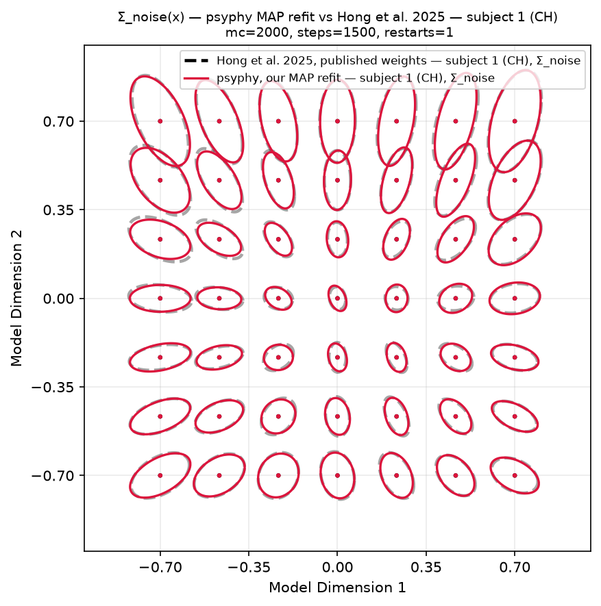
\(\Sigma_{\text{noise}}(x)\) for subject 1 (CH): dashed gray is the field from the authors' published weights, red is our own MAP refit. This is the paper's supplementary Figure S3.

Note: These ellipses look much like the ones at the top of the page, but they are a different quantity. \(\Sigma_{\text{noise}}(x) = U(x)U(x)^{\top} + \delta I\) is the covariance of the observer's internal representation at stimulus \(x\); the field the WPPM is parameterized in, read off at each grid point. No task enters it. The contours at the top are \(\Sigma_{\text{thres}}\), one step downstream: \(\Sigma_{\text{noise}}\) at a reference and a comparison feeds the oddity likelihood to give P(correct), and that map is inverted for the displacement at which P(correct) = 2/3. We use the same grid and plotting convention, but \(\Sigma_{\text{noise}}\) is the model's parameters evaluated, while \(\Sigma_{\text{thres}}\) is behavior predicted from them at a criterion, here 2/3.

---

End to end: from raw trials to Figure 2B

This is the figure at the top of the page, and this is where it comes from.

Each of the two steps before it held something fixed. The Figure 2B inversion started from the authors' published weights, so it tested our inversion. The refit went the other way: it fit weights from the raw trials, but only compared noise fields. Neither on its own shows that psyphy can get from raw data to the published figure, but they served individually as important implementation checks.

We now show that together psyphy can go:

raw trials -> fit weights -> derive threshold contours -> the published figure 2B

# The only line that differs from stage 2: the weights are ours.
W_fit = jnp.asarray(np.load(fit_path)["W"])

predictive = WPPMPredictivePosterior(
    MAPPosterior({"W": W_fit}, model),  # <- before we passed W_org here
    jnp.asarray(coords),
    n_samples=1,
    threshold_pred=True,
    threshold_config=thr["config"],
)
thres_fit = np.asarray(predictive.mean)  # (49, 2, 2)

Plotting it

Both contour fields go onto one axes in a single plot_ellipses call ( published dashed underneath, ours on top, each ellipse colored by its own reference stimulus)

plot_ellipses(
    coords,
    [Sigma_published, Sigma_psyphy],
    ax=ax,
    scale=scale,
    colors=["black", colors],
    linestyles=["--", "solid"],
    linewidths=[2.2, 1.6],
    alpha=[0.35, None],
    labels=[
        _published_label(subject),
        label or _ours_label(subject, "oddity inversion of their weights"),
    ],
    show_centers=True,
)

scale comes from auto_scale(coords, thres_published) and colors from hong2025.w2d_to_rgb(coords, M), the monitor calibration published with the data. For per-ellipse colors, posterior draws and the rest of the API, see Plotting ellipse fields.

66.7%-correct threshold contours for subject 1 (CH), computed from the weights we fit to the raw trials. There are no published weights anywhere in this chain. Dashed gray is the authors' published inversion; colored solid is ours, each ellipse taking the color of its reference stimulus.

---

Is that close enough? The paper's own bootstrap interval

How close is close enough? The authors answered that themselves. They resampled the trials 120 times, refit the model to each, and kept the 114 fits (95% of 120) that came out most like their original. The spread of those 114 contours is their 95% confidence interval and we check whether the threshold generated from psyphy's fit is comprised by that confidence interval in the figure below.

The figure below shows that our fit is indistinguishable from their run-to-run variaton at all 49 reference points and every direction tested, and in that sense psyphy's refit is indistinguishable from their fit.

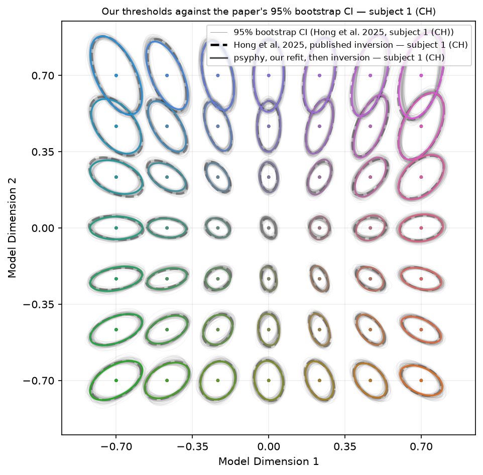
Our end-to-end contours against the paper's own 95% bootstrap interval for subject 1 (CH). The gray band is the 114 retained bootstrap refits, dashed gray the published fit, colored solid ours.

Plotting it:

plot_ellipses takes a whole stack of fields at once, so all 114 retained refits go on in a single call. The published fit and ours are drawn over them in the usual convention.

fig, ax = plt.subplots(figsize=(6.5, 6.5), dpi=150)

# Layer 1: the CI set. 114 fields in one call: plot_ellipses accepts a
# stack of shape (n_fields, n_points, 2, 2). thin and nearly transparent so
# they read as a band rather than distinguishable curves, and labelled
# once rather than n_field times
plot_ellipses(
    coords,
    boots,
    ax=ax,
    scale=scale,
    colors="0.55",
    linewidths=0.4,
    alpha=0.10,
    labels=[f"95% bootstrap CI (Hong et al. 2025, {_subject_tag(subject)})"]
    + [None] * (len(boots) - 1),
)
# Layer 2: the same convention for plotting as every other figure before
plot_ellipses(
    coords,
    [thres_published, thres_fit],
    ax=ax,
    scale=scale,
    colors=["black", colors],
    linestyles=["--", "solid"],
    linewidths=[2.2, 1.6],
    alpha=[0.35, None],
    labels=[
        _published_label(subject),
        _ours_label(subject, "our refit, then inversion"),
    ],
    show_centers=True,
)

Scope

These results are for one subject (CH, 1 of 8) and a single run on one GPU. They were not repeated for seed stability and not run for the other seven subjects. Read this as "the fitting pipeline reproduces the paper for this subject", not as a claim about all eight.

---

Runtimes

The full refit requires ~16 min on a single GPU. See the following table for a breakdown of how long each step takes.

Measured runtimes, step by step

CPU figures are an Apple Silicon laptop (M5); GPU is one A100 unless otherwise noted.

Step	Hardware	Wall clock	Details
Exact covariance check	CPU	seconds	10,609 points, deterministic
Thresholds, paper settings	CPU	~11 min	49 refs, n_theta=16, n_length=1000, mc=2000 (13.4 s per ref)
Thresholds, fast preset	CPU	20–23 s	n_length=300, mc=500 — smoke tests only
Refit — full	1 GPU	~8 min	6,000 trials, 1,500 steps, mc=2000, 3 restarts
The paper's own run	H100	14 h	one subject: main fit + 120 bootstrap refits

The 14-hour figure is per observer, not for the whole paper. The WPPM is fit separately for each participant, and the 120 bootstraps resample that participant's own trials, so all eight observers is roughly eight times that.

---

Watch out for

• \(\Sigma_{\text{noise}}\) and \(\Sigma_{\text{thres}}\) are different things. The thresholds above are \(\Sigma_{\text{thres}}\), as plotted in Figure 2B; the exact check and the refit compare \(\Sigma_{\text{noise}}\), the noise field, which is plotted in supplementary Figure S3. Both arrive as (49, 2, 2) stacks on the same grid, which makes them easy to conflate.
• The same seed gives the same answer on the same machine, but not necessarily on a different one. Re-running the inversion here is bit-identical: JAX's PRNG is deterministic given a key, so nothing changes between runs on the same machine. But what changes across machines is the floating-point arithmetic underneath: XLA reassociates or rewrite an expression, and a sum accumulated in a different order lands on a slightly different value (JAX FAQ). The exact check is unaffected, since it compares against a table rounded to 8 decimals. The thresholds and the refit can differ in their low-order digits between a laptop and a GPU
• Loss values are not comparable to the paper's. psyphy's Prior.log_prob drops a constant, which the paper keeps (still identical gradients but different numbers)

---

See also

• Full WPPM fit (simulated data) — more on the model math with ground truth available
• Quick start — the minimal version
• Plotting ellipse fields — plot_ellipses on its own, with synthetic data
• psyphy.data.published.hong2025 in Data; WPPMPredictivePosterior and ThresholdConfig in Posterior.