Fit your own data
This page is for readers who know the Wishart Process Psychophysical Model (WPPM) and want to fit it to their own trials with psyphy. It shows how psyphy stores trials and the calls in order, from a CSV file to thresholds and the checks we run on a fit. The model itself is explained in the WPPM tutorial.
We use one observer's published trials from Hong et al.: 12,000 oddity-task trials in a 2-D color plane. The script reads the number of stimulus dimensions from the data, so the same code fits 3-D stimuli.
The companion script is
fit_your_own_data.py.
The figures come from --mode full, Hong et al.'s Monte Carlo settings, run on 1 GPU.
How to run the script
The script downloads the trials from OSF the first time it runs (about 1 MB). We found no setting that converges within 10 min on a laptop CPU, so for your own data plan on a GPU.
Data in psyphy
psyphy keeps trials in a TrialData:
stimuli, shape(N, 2, d): \(N\) trials, 2 stimuli per trial, \(d\) stimulus dimensions. Slot 0 is the reference, slot 1 the comparison. The oddity task shows the reference twice, but psyphy stores it onceresponses, shape(N, 1): 1 for a correct response, 0 for an incorrect one
Every coordinate must lie in \([-1, 1]\), the domain of the Chebyshev basis. Rescale first, e.g.
2 * (x - lo) / (hi - lo) - 1. A fit doesn't check this. It returns a wrong field with no
error.
Hong et al.'s file has one row per trial and the columns TrialType, xref, x1 and y.
We read it with numpy:
The MOCS rows are trials at fixed comparison levels that Hong et al. didn't fit. We hold
them out for check (c). With your own data, hold out a random
subset instead, e.g. a fifth of the trials.
If your file has the columns ref, probe and response, with each stimulus written as a
list ("[0.1, -0.2]"),
load_responses_csv returns
the TrialData in one call.
Model
The prior settings are Hong et al.'s. For 3-D stimuli nothing in this code changes: d is
3, and the weights W get shape (5, 5, 5, 3, 4) instead of (5, 5, 2, 3). That is
Chebyshev degree 0 to 4 in each of the \(d\) stimulus dimensions, then \(d\), then \(d + 1\)
embedding dimensions.
GaussianNoise is required.
WPPM builds without it, but the fit then
raises an AttributeError that doesn't say what to pass.
Fit
MAPOptimizer starts from a
sample of the prior, picked by seed. We fit twice, from 2 prior samples, for
check (b).
| mode | steps | Monte Carlo samples per trial: fit, predictions | time for both fits |
|---|---|---|---|
quick |
300 | 20, 200 | 10 s, laptop CPU |
full |
1,500 | 2,000, 2,000 |
Results
The covariance field \(\Sigma(x)\) at the reference points we choose, here a 7 x 7 grid:
| The field at your reference points | |
|---|---|
For thresholds we predict with more Monte Carlo samples than we fit with. The predicted P(correct) is then less noisy.
| A model for predictions | |
|---|---|
WPPMPredictivePosterior
with threshold_pred=True searches n_theta directions around each reference for the
comparison that is correct 66.7% of the time, then fits an ellipse through those points (an
ellipsoid in 3-D).
More dimensions need more directions
In 2-D, 16 directions are enough, evenly spaced around the reference. From 3-D on, psyphy
picks the directions at random, and with 16 the ellipsoid misses the 66.7% contour in some
directions: P(correct) on it ranged from 0.48 to 0.97 in our check. With 64 it stayed
between 0.54 and 0.72. So raise n_theta as \(d\) grows (64 in 3-D costs ca. 4 times as
much as 16). It needs at least \(d(d+1)/2\).
plot_ellipses draws 2-D
ellipses. In 3-D we show the plane \(x_3 = 0\) and cut each ellipsoid with it:
The cut is the threshold for comparisons that stay in the plane. covs[:, :2, :2] is a
different ellipse: the ellipsoid's shadow on the plane, which is larger whenever the
ellipsoid is tilted out of it.
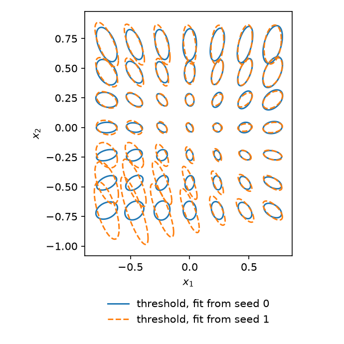
Threshold contours at 66.7% correct (thresholds above), not the noise
field covs, on a 7 x 7 grid of reference points. Solid: fit from seed 0.
Dashed: fit from seed 1. The 2 fits agree in the upper half and on the right. In the
lower left (x1 < 0, x2 < -0.25) the contours of seed 1 are larger and longer, so
there the 2 fits found different fields. Check
(a) shows why.
Checks with no ground truth
With your own data there's no true field to compare with. We check 3 things instead.
(a) The learning curve has flattened. The loss drops, then flattens into a noisy plateau. A curve that still trends down needs more steps, and spikes mean the fit hasn't settled.
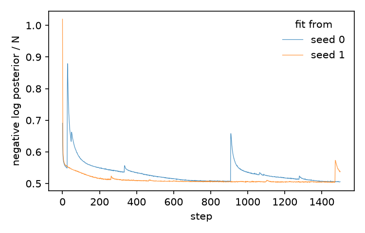
The loss MAPOptimizer minimizes, at each step: the negative log
posterior divided by the number of trials N, i.e. the negative log likelihood plus the
negative log prior, per trial. One line per fit. Both drop within the first 50 steps
and flatten near 0.51. Each spike is a step that jumped away from the plateau, and the
loss comes back down after it. The last spike of seed 1, at ca. step 1,470, hasn't come
back down by the final step.
MAPOptimizer returns the parameters of the final step. A curve that ends on a spike
therefore returns a fit from inside the spike, as seed 1 does here. Run more steps, or fit
again from another seed. A flat curve alone doesn't show convergence either, since a fit can
sit on a plateau above the optimum. So we also run (b).
(b) 2 fits from different prior samples give the same field. We compare the thresholds of the 2 fits point by point, as the relative Frobenius distance \(\lVert \Sigma_1 - \Sigma_0 \rVert_F / \lVert \Sigma_0 \rVert_F\):
| Compare the 2 fits | |
|---|---|
For a converged fit this is close to 0 at every point. A value near 1 means the 2 fits found different fields, as in the lower left of the threshold figure above.
(c) The fit predicts trials it wasn't fitted on. We sort the held-out trials into 10 bins by predicted P(correct), and compare each bin's mean prediction with the proportion of correct responses in it:
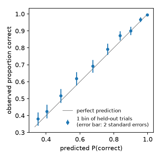
Fit from seed 0, on the 6,000 held-out trials. One dot per bin of 600 trials, with 2 standard errors. Gray: perfect prediction. The dots follow the diagonal from a predicted P(correct) of 0.35 to 1, and the error bars of most bins cross it, so the fit predicts trials it wasn't fitted on. 2 bins, near 0.58 and 0.84, sit just above it.
The dots should lie on the diagonal, within their error bars. Dots above it mean the fit predicts too few correct responses, dots below too many.
If you simulated your data
With a known field, compare the fit with it directly. Here we use Hong et al.'s
published fit in place of a ground truth, loaded with
load_reference_W:
For your simulation, pass your true W in place of W_published, in the shape
prior gives it. load_reference_W reads 2-D weights only. If your simulation
returns \(\Sigma\) at the reference points instead, compare covs with those.
Next steps
- Sampling the posterior with NUTS, for uncertainty on the thresholds instead of a single fit
- Reproducing Hong et al. (2025), the full refit of the paper
- questions and bugs: GitHub issues