Introduction to GLM

Introduction to GLM#

This notebook has had all its explanatory text removed and has not been run. It is intended to be downloaded and run locally (or on the provided binder) while listening to the presenter’s explanation. In order to see the fully rendered of this notebook, go here

Data for this notebook is a patch clamp experiment with a mouse V1 neuron, from the Allen Brain Atlas

Allen Brain Atlas view of the data we will analyze.

Learning objectives#

Learn how to explore spiking data and do basic analyses using pynapple
Learn how to structure data for NeMoS
Learn how to fit a basic Generalized Linear Model using NeMoS
Learn how to retrieve the parameters and predictions from a fit GLM for intrepetation.

# Import everything
import jax
import matplotlib.pyplot as plt
import numpy as np
import pynapple as nap

import nemos as nmo

# some helper plotting functions
from nemos import _documentation_utils as doc_plots
import workshop_utils

# configure plots some
plt.style.use(nmo.styles.plot_style)

Data Streaming#

Stream the data. Format is Neurodata Without Borders (NWB) standard

path = workshop_utils.fetch_data("allen_478498617.nwb")

Pynapple#

Data structures and preparation#

Open the NWB file with pynapple

data = nap.load_file(path)
print(data)

Annotated view of the data we will analyze.

stimulus: injected current, in Amperes, sampled at 20k Hz.
response: the neuron’s intracellular voltage, sampled at 20k Hz. We will not use this info in this example.
units: dictionary of neurons, holding each neuron’s spike timestamps.
epochs: start and end times of different intervals, defining the experimental structure, specifying when each stimulation protocol began and ended.

trial_interval_set = data["epochs"]

current = data["stimulus"]
spikes = data["units"]

trial_interval_set

Noise 1: epochs of random noise

noise_interval = trial_interval_set[trial_interval_set.tags == "Noise 1"]
noise_interval

Let’s focus on the first epoch.

noise_interval = noise_interval[0]
noise_interval

current : Tsd (TimeSeriesData) : time index + data

current

restrict : restricts a time series object to a set of time intervals delimited by an IntervalSet object

current = current.restrict(noise_interval)
# convert current from Ampere to pico-amperes, to match the above visualization
# and move the values to a more reasonable range.
current = current * 1e12
current

TsGroup : a dictionary-like object holding multiple Ts (timeseries) objects with potentially different time indices.

spikes

We can index into the TsGroup to see the timestamps for this neuron’s spikes:

spikes[0]

Let’s restrict to the same epoch noise_interval:

spikes = spikes.restrict(noise_interval)
print(spikes)
spikes[0]

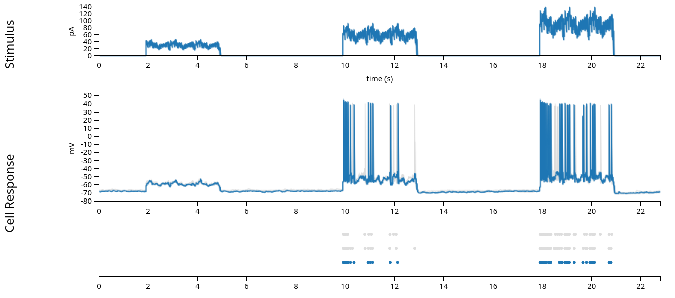
Let’s visualize the data from this trial:

fig, ax = plt.subplots(1, 1, figsize=(8, 2))
ax.plot(current, "grey")
ax.plot(spikes.to_tsd([-5]), "|", color="k", ms = 10)
ax.set_ylabel("Current (pA)")
ax.set_xlabel("Time (s)")

Basic analyses#

The Generalized Linear Model gives a predicted firing rate. First we can use pynapple to visualize this firing rate for a single trial.

count : count the number of events within bin_size

# bin size in seconds
bin_size = 0.001
# Get spikes for neuron 0
count = spikes[0].count(bin_size)
count

Let’s convert the spike counts to firing rate :

smooth : convolve with a Gaussian kernel

# the inputs to this function are the standard deviation of the gaussian in seconds and
# the full width of the window, in standard deviations. So std=.05 and size_factor=20
# gives a total filter size of 0.05 sec * 20 = 1 sec.
firing_rate = count.smooth(std=0.05, size_factor=20)
# convert from spikes per bin to spikes per second (Hz)
firing_rate = firing_rate / bin_size

print(type(firing_rate))

doc_plots.current_injection_plot(current, spikes, firing_rate);

What is the relationship between the current and the spiking activity? compute_1d_tuning_curves : compute the firing rate as a function of a 1-dimensional feature.

tuning_curve = nap.compute_1d_tuning_curves(spikes, current, nb_bins=15)
tuning_curve

Let’s plot the tuning curve of the neuron.

doc_plots.tuning_curve_plot(tuning_curve);

NeMoS#

Preparing data#

Get data from pynapple to NeMoS-ready format:

predictors and spikes must have same number of time points

binned_current = current.bin_average(bin_size)

print(f"current shape: {binned_current.shape}")
# rate is in Hz, convert to KHz
print(f"current sampling rate: {binned_current.rate/1000.:.02f} KHz")

print(f"\ncount shape: {count.shape}")
print(f"count sampling rate: {count.rate/1000:.02f} KHz")

predictors must be 2d, spikes 1d

predictor = np.expand_dims(binned_current, 1)

# check that the dimensionality matches NeMoS expectation
print(f"predictor shape: {predictor.shape}")
print(f"count shape: {count.shape}")

Fitting the model#

GLM objects need regularizers and observation models

# Initialize the model, specifying the solver. we'll accept the defaults
# for everything else.
model = nmo.glm.GLM(solver_name="LBFGS")

call fit and retrieve parameters

model.fit(predictor, count)

print(f"firing_rate(t) = exp({model.coef_} * current(t) + {model.intercept_})")

print(f"coef_ shape: {model.coef_.shape}")
print(f"intercept_ shape: {model.intercept_.shape}")

generate and examine model predictions.

predicted_fr = model.predict(predictor)
# convert units from spikes/bin to spikes/sec
predicted_fr = predicted_fr / bin_size


# and let's smooth the firing rate the same way that we smoothed the firing rate
smooth_predicted_fr = predicted_fr.smooth(0.05, size_factor=20)

# and plot!
fig = doc_plots.current_injection_plot(current, spikes, firing_rate,
                                 # plot the predicted firing rate that has
                                 # been smoothed the same way as the
                                 # smoothed spike train
                                 predicted_firing_rate=smooth_predicted_fr)

what do we see?

# compare observed mean firing rate with the model predicted one
print(f"Observed mean firing rate: {np.mean(count) / bin_size} Hz")
print(f"Predicted mean firing rate: {np.mean(predicted_fr)} Hz")

examine tuning curve — what do we see?

# pynapple expects the input to this function to be 2d,
# so let's add a singleton dimension
tuning_curve_model = nap.compute_1d_tuning_curves_continuous(predicted_fr[:, np.newaxis], current, 15)
fig = doc_plots.tuning_curve_plot(tuning_curve)
fig.axes[0].plot(tuning_curve_model, color="tomato", label="glm")
fig.axes[0].legend()

Extending the model to use injection history#

choose a length of time over which the neuron integrates the input current

current_history_duration_sec = .2
# convert this from sec to bins
current_history_duration = int(current_history_duration_sec / bin_size)

binned_current[1:]
binned_current[2:]
# etc

doc_plots.plot_basis();

define a basis object

basis = nmo.basis.RaisedCosineLogConv(
    n_basis_funcs=8, window_size=current_history_duration,
)

create the design matrix
examine the features it contains

# under the hood, this convolves the input with the filter bank visualized above
current_history = basis.compute_features(binned_current)
print(current_history)

# in this plot, we're normalizing the amplitudes to make the comparison easier --
# the amplitude of these features will be fit by the model, so their un-scaled
# amplitudes is not informative
workshop_utils.plot_current_history_features(binned_current, current_history, basis,
                                             current_history_duration_sec)

create and fit the GLM
examine the parameters

history_model = nmo.glm.GLM(solver_name="LBFGS")
history_model.fit(current_history, count)

print(f"firing_rate(t) = exp({history_model.coef_} * current(t) + {history_model.intercept_})")

print(history_model.coef_.shape)
print(history_model.intercept_.shape)

Visualize the current history model’s learned filter.
This filter is convolved with the input current and used to predict the firing rate.

workshop_utils.plot_basis_filter(basis, history_model)

compare the predicted firing rate to the data and the old model
what do we see?

# all this code is the same as above
history_pred_fr = history_model.predict(current_history)
history_pred_fr = history_pred_fr / bin_size
smooth_history_pred_fr = history_pred_fr.dropna().smooth(.05, size_factor=20)
workshop_utils.current_injection_plot(current, spikes, firing_rate,
                                      # compare against the old firing rate
                                      smooth_history_pred_fr, smooth_predicted_fr)

examine the predicted average firing rate and tuning curve
what do we see?

# compare observed mean firing rate with the history_model predicted one
print(f"Observed mean firing rate: {np.mean(count) / bin_size} Hz")
print(f"Predicted mean firing rate (instantaneous current): {np.nanmean(predicted_fr)} Hz")
print(f"Predicted mean firing rate (current history): {np.nanmean(smooth_history_pred_fr)} Hz")

# Visualize tuning curve
tuning_curve_history_model = nap.compute_1d_tuning_curves_continuous(smooth_history_pred_fr, current, 15)
fig = doc_plots.tuning_curve_plot(tuning_curve)
fig.axes[0].plot(tuning_curve_history_model, color="tomato", label="glm (current history)")
fig.axes[0].plot(tuning_curve_model, color="tomato", linestyle='--', label="glm (instantaneous current)")
fig.axes[0].legend()

use log-likelihood to compare models

log_likelihood = model.score(predictor, count, score_type="log-likelihood")
print(f"log-likelihood (instantaneous current): {log_likelihood}")
log_likelihood = history_model.score(current_history, count, score_type="log-likelihood")
print(f"log-likelihood (current history): {log_likelihood}")

Finishing up#

what if you want to compare models across datasets?

r2 = model.score(predictor, count, score_type='pseudo-r2-Cohen')
print(f"pseudo-r2 (instantaneous current): {r2}")
r2 = history_model.score(current_history, count, score_type='pseudo-r2-Cohen')
print(f"pseudo-r2 (current history): {r2}")

Further Exercises#

what else can we do?

Data citation#

The data used in this tutorial is from the Allen Brain Map, with the following citation:

Contributors: Agata Budzillo, Bosiljka Tasic, Brian R. Lee, Fahimeh Baftizadeh, Gabe Murphy, Hongkui Zeng, Jim Berg, Nathan Gouwens, Rachel Dalley, Staci A. Sorensen, Tim Jarsky, Uygar Sümbül Zizhen Yao

Dataset: Allen Institute for Brain Science (2020). Allen Cell Types Database – Mouse Patch-seq [dataset]. Available from brain-map.org/explore/classes/multimodal-characterization.

Primary publication: Gouwens, N.W., Sorensen, S.A., et al. (2020). Integrated morphoelectric and transcriptomic classification of cortical GABAergic cells. Cell, 183(4), 935-953.E19. https://doi.org/10.1016/j.cell.2020.09.057

Patch-seq protocol: Lee, B. R., Budzillo, A., et al. (2021). Scaled, high fidelity electrophysiological, morphological, and transcriptomic cell characterization. eLife, 2021;10:e65482. https://doi.org/10.7554/eLife.65482