Show code cell source Hide code cell source

%load_ext autoreload
%autoreload 2

%matplotlib inline
import warnings

warnings.filterwarnings(
    "ignore",
    message="plotting functions contained within `_documentation_utils` are intended for nemos's documentation.",
    category=UserWarning,
)

warnings.filterwarnings(
    "ignore",
    message="Ignoring cached namespace 'core'",
    category=UserWarning,
)

warnings.filterwarnings(
    "ignore",
    message=(
        "invalid value encountered in div "
    ),
    category=RuntimeWarning,
)

Download

This notebook can be downloaded as place_cells.ipynb. See the button at the top right to download as markdown or pdf.

Model and feature selection with scikit-learn

Data for this notebook comes from recordings in the mouse hippocampus while the mouse runs on a linear track. We explored this data yesterday. Today, we will see that the neurons present in this recording show both tuning for both speed and location (i.e., place fields). However, location and speed are highly correlated. We would like to know which feature is more informative for predicting neuronal firing rate — how do we do that?

Data for this notebook comes from recordings in the mouse hippocampus while the mouse runs on a linear track, which we [explored yesterday](../day1/phase_precession-users.md).

Learning objectives

• Review how to use pynapple to analyze neuronal tuning

• Learn how to combine NeMoS basis objects

• Learn how to use NeMoS objects with scikit-learn for cross-validation

• Learn how to use NeMoS objects with scikit-learn pipelines

• Learn how to use cross-validation to perform model and feature selection

import matplotlib.pyplot as plt
import numpy as np
import pandas as pd
import pynapple as nap

import nemos as nmo

# some helper plotting functions
from nemos import _documentation_utils as doc_plots
import workshop_utils

# configure plots some
plt.style.use(nmo.styles.plot_style)

import workshop_utils

from sklearn import model_selection
from sklearn import pipeline

# shut down jax to numpy conversion warning
nap.nap_config.suppress_conversion_warnings = True

# during development, set this to a lower number so everything runs faster. 
cv_folds = 5

WARNING:2025-02-04 19:33:50,036:jax._src.xla_bridge:987: An NVIDIA GPU may be present on this machine, but a CUDA-enabled jaxlib is not installed. Falling back to cpu.

Pynapple

- Load the data using pynapple.

path = workshop_utils.fetch_data("Achilles_10252013_EEG.nwb")
data = nap.load_file(path)
data

/home/agent/workspace/rorse_ccn-software-jan-2025_main/lib/python3.11/site-packages/hdmf/spec/namespace.py:535: UserWarning: Ignoring cached namespace 'hdmf-common' version 1.7.0 because version 1.8.0 is already loaded.
  warn("Ignoring cached namespace '%s' version %s because version %s is already loaded."
/home/agent/workspace/rorse_ccn-software-jan-2025_main/lib/python3.11/site-packages/hdmf/spec/namespace.py:535: UserWarning: Ignoring cached namespace 'hdmf-experimental' version 0.4.0 because version 0.5.0 is already loaded.
  warn("Ignoring cached namespace '%s' version %s because version %s is already loaded."

Achilles_10252013_EEG
┍━━━━━━━━━━━━━┯━━━━━━━━━━━━━┑
│ Keys        │ Type        │
┝━━━━━━━━━━━━━┿━━━━━━━━━━━━━┥
│ units       │ TsGroup     │
│ rem         │ IntervalSet │
│ nrem        │ IntervalSet │
│ forward_ep  │ IntervalSet │
│ eeg         │ TsdFrame    │
│ theta_phase │ Tsd         │
│ position    │ Tsd         │
┕━━━━━━━━━━━━━┷━━━━━━━━━━━━━┙

- Extract the spike times and mouse position.

spikes = data["units"]
position = data["position"]

For today, we’re only going to focus on the times when the animal was traversing the linear track. This is a pynapple IntervalSet, so we can use it to restrict our other variables:

• Restrict data to when animal was traversing the linear track.

position = position.restrict(data["forward_ep"])
spikes = spikes.restrict(data["forward_ep"])

The recording contains both inhibitory and excitatory neurons. Here we will focus of the excitatory cells with firing above 0.3 Hz.

• Restrict neurons to only excitatory neurons, discarding neurons with a low-firing rate.

spikes = spikes.getby_category("cell_type")["pE"]
spikes = spikes.getby_threshold("rate", 0.3)

Place fields

By plotting the neuronal firing rate as a function of position, we can see that these neurons are all tuned for position: they fire in a specific location on the track.

• Visualize the place fields: neuronal firing rate as a function of position.

place_fields = nap.compute_1d_tuning_curves(spikes, position, 50, position.time_support)
workshop_utils.plot_place_fields(place_fields)

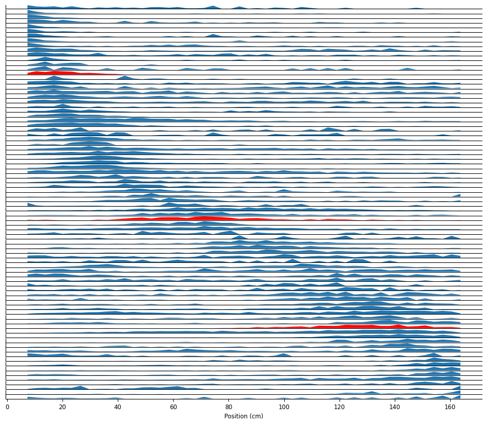
To decrease computation time, we’re going to spend the rest of the notebook focusing on the neurons highlighted above. We’re also going to bin spikes at 100 Hz and up-sample the position to match that temporal resolution.

• For speed, we’re only going to investigate the three neurons highlighted above.

• Bin spikes to counts at 100 Hz.

• Interpolate position to match spike resolution.

neurons = [82, 92, 220]
place_fields = place_fields[neurons]
spikes = spikes[neurons]
bin_size = .01
count = spikes.count(bin_size, ep=position.time_support)
position = position.interpolate(count, ep=count.time_support)
print(count.shape)
print(position.shape)

(19237, 3)
(19237,)

Speed modulation

The speed at which the animal traverse the field is not homogeneous. Does it influence the firing rate of hippocampal neurons? We can compute tuning curves for speed as well as average speed across the maze. In the next block, we compute the speed of the animal for each epoch (i.e. crossing of the linear track) by doing the difference of two consecutive position multiplied by the sampling rate of the position.

• Compute animal’s speed for each epoch.

speed = []
# Analyzing each epoch separately avoids edge effects.
for s, e in position.time_support.values: 
    pos_ep = position.get(s, e)
    # Absolute difference of two consecutive points
    speed_ep = np.abs(np.diff(pos_ep)) 
    # Padding the edge so that the size is the same as the position/spike counts
    speed_ep = np.pad(speed_ep, [0, 1], mode="edge") 
    # Converting to cm/s 
    speed_ep = speed_ep * position.rate
    speed.append(speed_ep)

speed = nap.Tsd(t=position.t, d=np.hstack(speed), time_support=position.time_support)
print(speed.shape)

(19237,)

Now that we have the speed of the animal, we can compute the tuning curves for speed modulation. Here we call pynapple compute_1d_tuning_curves:

• Compute the tuning curve with pynapple’s compute_1d_tuning_curves

tc_speed = nap.compute_1d_tuning_curves(spikes, speed, 20, speed.time_support)

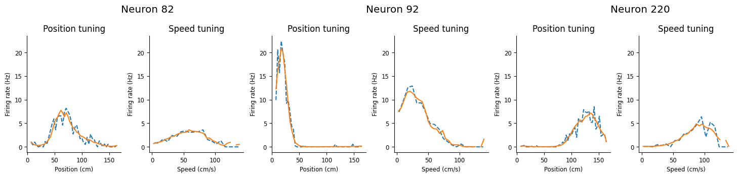
• Visualize the position and speed tuning for these neurons.

fig = workshop_utils.plot_position_speed(position, speed, place_fields, tc_speed, neurons);

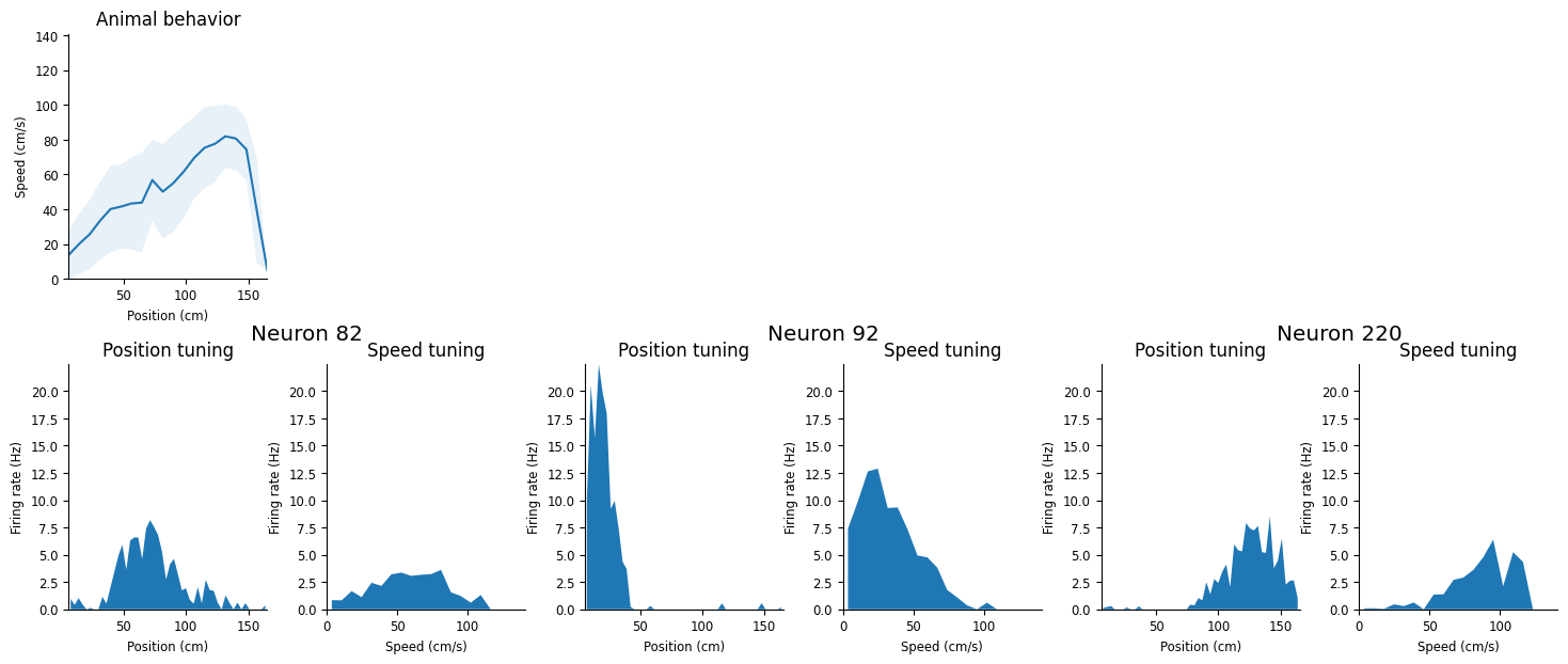
These neurons show a strong modulation of firing rate as a function of speed but we also notice that the animal, on average, accelerates when traversing the field. Is the speed tuning we observe a true modulation or spurious correlation caused by traversing the place field at different speeds? We can use NeMoS to model the activity and give the position and the speed as input variable.

These neurons all show both position and speed tuning, and we see that the animal’s speed and position are highly correlated. We’re going to build a GLM to predict neuronal firing rate – which variable should we use? Is the speed tuning just epiphenomenal?

NeMoS

Basis evaluation

As we’ve seen before, we will use basis objects to represent the input values. In previous tutorials, we’ve used the Conv basis objects to represent the time-dependent effects we were looking to capture. Here, we’re trying to capture the non-linear relationship between our input variables and firing rate, so we want the Eval objects. In these circumstances, you should look at the tuning you’re trying to capture and compare to the basis kernels (visualized in NeMoS docs): you want your tuning to be capturable by a linear combination of them.

In this case, several of these would probably work; we will use MSplineEval for both, though with different numbers of basis functions.

Additionally, since we have two different inputs, we’ll need two separate basis objects.

Note

Later in this notebook, we’ll show how to cross-validate across basis identity, which you can use to choose the basis.

• why basis?

  • without basis:

    • either the GLM says that firing rate increases exponentially as position or speed increases, which is fairly nonsensical,

    • or we have to fit the weight separately for each position or speed, which is really high-dim

  • so, basis allows us to reduce dimensionality, capture non-linear modulation of firing rate (in this case, tuning)

• why eval?

  • basis objects have two modes:

  • conv, like we’ve seen, for capturing time-dependent effects

  • eval, for capturing non-linear modulation / tuning

• why MSpline?

  • when deciding on eval basis, look at the tuning you want to capture, compare to the kernels: you want your tuning to be capturable by a linear combination of these

  • in cases like this, many possible basis objects we could use here and what I’ll show you in a bit will allow you to determine which to use in principled manner

  • MSpline, BSpline, RaisedCosineLinear : all would let you capture this

  • weird choices:

    • cyclic bspline, except maybe for position? if end and start are the same

    • RaisedCosineLog (don’t want the stretching)

    • orthogonalized exponential (specialized for…)

    • identity / history (too basic)

• Create a separate basis object for each model input.

• Visualize the basis objects.

position_basis = nmo.basis.MSplineEval(n_basis_funcs=10)
speed_basis = nmo.basis.MSplineEval(n_basis_funcs=15)
workshop_utils.plot_pos_speed_bases(position_basis, speed_basis)

However, now we have an issue: in all our previous examples, we had a single basis object, which took a single input to produce a single array which we then passed to the GLM object as the design matrix. What do we do when we have multiple basis objects?

We could call basis.compute_features() for each basis separately and then concatenated the outputs, but then we have to remember the order we concatenated them in and that behavior gets unwieldy as we add more bases.

Instead, NeMoS allows us to combine multiple basis objects into a single “additive basis”, which we can pass all of our inputs to in order to produce a single design matrix:

• Combine the two basis objects into a single “additive basis”

# equivalent to calling nmo.basis.AdditiveBasis(position_basis, speed_basis)
basis = position_basis + speed_basis

• Create the design matrix!

• Notice that, since we passed the basis pynapple objects, we got one back, preserving the time stamps.

• X has the same number of time points as our input position and speed, but 25 columns. The columns come from n_basis_funcs from each basis (10 for position, 15 for speed).

X = basis.compute_features(position, speed)
X

Time (s)         0        1        2        3    4    ...
---------------  -------  -------  -------  ---  ---  -----
18193.603802655  0.16285  0.0063   5e-05    0.0  0.0  ...
18193.613802655  0.15956  0.0079   9e-05    0.0  0.0  ...
18193.623802655  0.1563   0.00947  0.00012  0.0  0.0  ...
18193.633802655  0.15111  0.01195  0.0002   0.0  0.0  ...
18193.643802655  0.1459   0.0144   0.0003   0.0  0.0  ...
18193.653802655  0.14197  0.01623  0.00039  0.0  0.0  ...
18193.663802655  0.13996  0.01716  0.00045  0.0  0.0  ...
...              ...      ...      ...      ...  ...  ...
20123.332682821  0.0      0.0      0.0      0.0  0.0  ...
20123.342682821  0.0      0.0      0.0      0.0  0.0  ...
20123.352682821  0.0      0.0      0.0      0.0  0.0  ...
20123.362682821  0.0      0.0      0.0      0.0  0.0  ...
20123.372682821  0.0      0.0      0.0      0.0  0.0  ...
20123.382682821  0.0      0.0      0.0      0.0  0.0  ...
20123.392682821  0.0      0.0      0.0      0.0  0.0  ...
dtype: float64, shape: (19237, 25)

Model learning

As we’ve done before, we can now use the Poisson GLM from NeMoS to learn the combined model:

• Initialize PopulationGLM

• Use the “LBFGS” solver and pass {"tol": 1e-12} to solver_kwargs.

• Fit the data, passing the design matrix and spike counts to the glm object.

# initialize 
glm =

# and fit

glm = nmo.glm.PopulationGLM(
    solver_kwargs={"tol": 1e-12},
    solver_name="LBFGS",
)

glm.fit(X, count)

PopulationGLM(
    observation_model=PoissonObservations(inverse_link_function=exp),
    regularizer=UnRegularized(),
    solver_name='LBFGS',
    solver_kwargs={'tol': 1e-12}
)

Prediction

Let’s check first if our model can accurately predict the tuning curves we displayed above. We can use the predict function of NeMoS and then compute new tuning curves

• Use predict to check whether our GLM has captured each neuron’s speed and position tuning.

• Remember to convert the predicted firing rate to spikes per second!

# predict the model's firing rate
predicted_rate = 

# same shape as the counts we were trying to predict
print(predicted_rate.shape, count.shape)

# compute the position and speed tuning curves using the predicted firing rate.
glm_pos = 
glm_speed = 

# predict the model's firing rate
predicted_rate = glm.predict(X) / bin_size

# same shape as the counts we were trying to predict
print(predicted_rate.shape, count.shape)

# compute the position and speed tuning curves using the predicted firing rate.
glm_pos = nap.compute_1d_tuning_curves_continuous(predicted_rate, position, 50, position.time_support)
glm_speed = nap.compute_1d_tuning_curves_continuous(predicted_rate, speed, 30, speed.time_support)

(19237, 3) (19237, 3)

/home/agent/workspace/rorse_ccn-software-jan-2025_main/lib/python3.11/site-packages/numpy/_core/fromnumeric.py:3904: RuntimeWarning: Mean of empty slice.
  return _methods._mean(a, axis=axis, dtype=dtype,
/home/agent/workspace/rorse_ccn-software-jan-2025_main/lib/python3.11/site-packages/numpy/_core/_methods.py:139: RuntimeWarning: invalid value encountered in divide
  ret = um.true_divide(

• Compare model and data tuning curves together. The model did a pretty good job!

workshop_utils.plot_position_speed_tuning(place_fields, tc_speed, glm_pos, glm_speed);

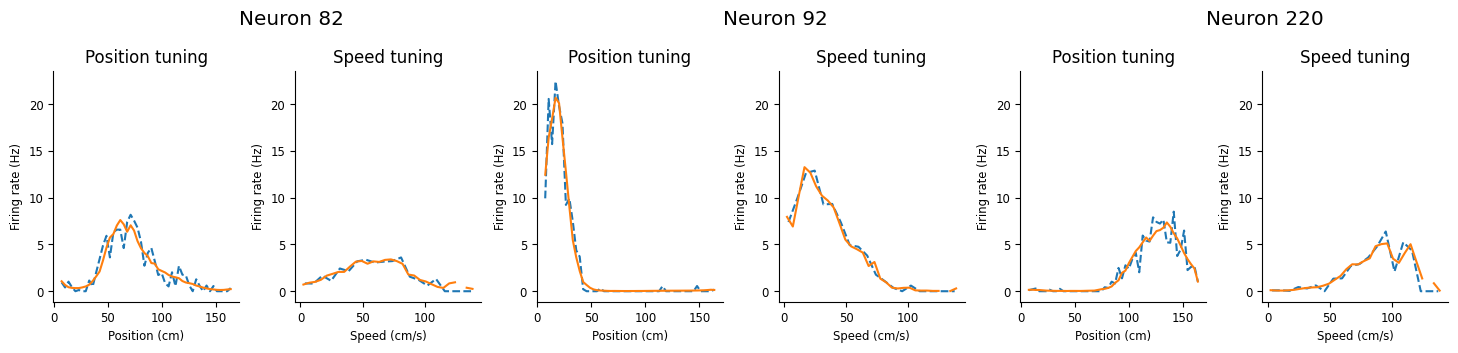
We can see that this model does a good job capturing both the position and the speed. In the rest of this notebook, we’re going to investigate all the scientific decisions that we swept under the rug: should we regularize the model? what basis should we use? do we need both inputs?

To make our lives easier, let’s create a helper function that wraps the above lines, because we’re going to be visualizing our model predictions a lot.

def visualize_model_predictions(glm, X):
    # predict the model's firing rate
    predicted_rate = glm.predict(X) / bin_size

    # compute the position and speed tuning curves using the predicted firing rate.
    glm_pos = nap.compute_1d_tuning_curves_continuous(predicted_rate, position, 50, position.time_support)
    glm_speed = nap.compute_1d_tuning_curves_continuous(predicted_rate, speed, 30, position.time_support)

    workshop_utils.plot_position_speed_tuning(place_fields, tc_speed, glm_pos, glm_speed);

Scikit-learn

How to know when to regularize?

In the last session, Edoardo fit the all-to-all connectivity of the head-tuning dataset using the Ridge regularizer. In the model above, we’re not using any regularization? Why is that?

We have far fewer parameters here then in the last example. However, how do you know if you need regularization or not? One thing you can do is use cross-validation to see whether model performance improves with regularization (behind the scenes, this is what we did!). We’ll walk through how to do that now.

Instead of implementing our own cross-validation machinery, the developers of nemos decided that we should write the package to be compliant with scikit-learn, the canonical machine learning python library. Our models are all what scikit-learn calls “estimators”, which means they have .fit, .score. and .predict methods. Thus, we can use them with scikit-learn’s objects out of the box.

We’re going to use scikit-learn’s GridSearchCV object, which performs a cross-validated grid search, as Edoardo explained in his presentation.

This object requires an estimator, our glm object here, and param_grid, a dictionary defining what to check. For now, let’s just compare Ridge regularization with no regularization:

• How do we decide when to use regularization?

• Cross-validation allows you to fairly compare different models on the same dataset.

• NeMoS makes use of scikit-learn, the standard machine learning library in python.

• Define parameter grid to search over.

• Anything not specified in grid will be kept constant.

param_grid = {
    "regularizer": ["UnRegularized", "Ridge"],
}

• Initialize scikit-learn’s GridSearchCV object.

cv = model_selection.GridSearchCV(glm, param_grid, cv=cv_folds)
cv

GridSearchCV(cv=5,
             estimator=PopulationGLM(
    observation_model=PoissonObservations(inverse_link_function=exp),
    regularizer=UnRegularized(),
    solver_name='LBFGS',
    solver_kwargs={'tol': 1e-12}
),
             param_grid={'regularizer': ['UnRegularized', 'Ridge']})

In a Jupyter environment, please rerun this cell to show the HTML representation or trust the notebook.
On GitHub, the HTML representation is unable to render, please try loading this page with nbviewer.org.

This will take a bit to run, because we’re fitting the model many times!

• We interact with this in a very similar way to the glm object.

• In particular, call fit with same arguments:

cv.fit(X, count)

/home/agent/workspace/rorse_ccn-software-jan-2025_main/lib/python3.11/site-packages/nemos/base_regressor.py:193: UserWarning: Caution: regularizer strength has not been set. Defaulting to 1.0. Please see the documentation for best practices in setting regularization strength.
  warnings.warn(

/home/agent/workspace/rorse_ccn-software-jan-2025_main/lib/python3.11/site-packages/nemos/base_regressor.py:193: UserWarning: Caution: regularizer strength has not been set. Defaulting to 1.0. Please see the documentation for best practices in setting regularization strength.
  warnings.warn(

/home/agent/workspace/rorse_ccn-software-jan-2025_main/lib/python3.11/site-packages/nemos/base_regressor.py:193: UserWarning: Caution: regularizer strength has not been set. Defaulting to 1.0. Please see the documentation for best practices in setting regularization strength.
  warnings.warn(

/home/agent/workspace/rorse_ccn-software-jan-2025_main/lib/python3.11/site-packages/nemos/base_regressor.py:193: UserWarning: Caution: regularizer strength has not been set. Defaulting to 1.0. Please see the documentation for best practices in setting regularization strength.
  warnings.warn(

/home/agent/workspace/rorse_ccn-software-jan-2025_main/lib/python3.11/site-packages/nemos/base_regressor.py:193: UserWarning: Caution: regularizer strength has not been set. Defaulting to 1.0. Please see the documentation for best practices in setting regularization strength.
  warnings.warn(

GridSearchCV(cv=5,
             estimator=PopulationGLM(
    observation_model=PoissonObservations(inverse_link_function=exp),
    regularizer=UnRegularized(),
    solver_name='LBFGS',
    solver_kwargs={'tol': 1e-12}
),
             param_grid={'regularizer': ['UnRegularized', 'Ridge']})

In a Jupyter environment, please rerun this cell to show the HTML representation or trust the notebook.
On GitHub, the HTML representation is unable to render, please try loading this page with nbviewer.org.

• We got a warning because we didn’t specify the regularizer strength, so we just fell back on default value.

• Let’s investigate results:

Cross-validation results are stored in a dictionary attribute called cv_results_, which contains a lot of info.

cv.cv_results_

{'mean_fit_time': array([2.34017291, 2.00892472]),
 'std_fit_time': array([0.42876242, 0.1954901 ]),
 'mean_score_time': array([0.18504963, 0.00365276]),
 'std_score_time': array([0.22262815, 0.00041068]),
 'param_regularizer': masked_array(data=['UnRegularized', 'Ridge'],
              mask=[False, False],
        fill_value=np.str_('?'),
             dtype=object),
 'params': [{'regularizer': 'UnRegularized'}, {'regularizer': 'Ridge'}],
 'split0_test_score': array([-0.11310252, -0.13712785]),
 'split1_test_score': array([-0.10429042, -0.12844072]),
 'split2_test_score': array([-0.13868614, -0.17322585]),
 'split3_test_score': array([-0.11728746, -0.13869132]),
 'split4_test_score': array([-0.11506688, -0.1312802 ]),
 'mean_test_score': array([-0.11768668, -0.14175319]),
 'std_test_score': array([0.01138836, 0.01617531]),
 'rank_test_score': array([1, 2], dtype=int32)}

The most informative for us is the 'mean_test_score' key, which shows the average of glm.score on each test-fold. Thus, higher is better, and we can see that the UnRegularized model performs better.

Note

You could (and generally, should!) investigate regularizer_strength, but we’re skipping for simplicity. To do this properly, use a slightly different syntax for param_grid (list of dictionaries, instead of single dictionary)

param_grid = [
    {"regularizer": [nmo.regularizer.UnRegularized()]},
    {"regularizer": [nmo.regularizer.Ridge()],
     "regularizer_strength": [1e-6, 1e-3, 1]}
]

Select basis

We can do something similar to select the basis. In the above example, I just told you which basis function to use and how many of each. But, in general, you want to select those in a reasonable manner. Cross-validation to the rescue!

Unlike the glm objects, our basis objects are not scikit-learn compatible right out of the box. However, they can be made compatible by using the .to_transformer() method (or, equivalently, by using the TransformerBasis class)

• You can (and should) do something similar to determine how many basis functions you need for each input.

• NeMoS basis objects are not scikit-learn-compatible right out of the box.

• But we have provided a simple method to make them so:

position_basis = nmo.basis.MSplineEval(n_basis_funcs=10).to_transformer()
# or equivalently:
position_basis = nmo.basis.TransformerBasis(nmo.basis.MSplineEval(n_basis_funcs=10))

This gives the basis object the transform method, which is equivalent to compute_features. However, transformers have some limits:

• This gives the basis object the transform method, which is equivalent to compute_features.

• However, transformers have some limits:

position_basis.transform(position)

---------------------------------------------------------------------------
RuntimeError                              Traceback (most recent call last)
Cell In[24], line 1
----> 1 position_basis.transform(position)

File ~/lib/python3.11/site-packages/nemos/basis/_transformer_basis.py:202, in TransformerBasis.transform(self, X, y)
    165 def transform(self, X: FeatureMatrix, y=None) -> FeatureMatrix:
    166     """
    167     Transform the data using the fitted basis functions.
    168 
   (...)
    200     >>> feature_transformed = transformer.transform(X)
    201     """
--> 202     self._check_initialized(self.basis)
    203     self._check_input(X, y)
    204     # transpose does not work with pynapple
    205     # can't use func(*X.T) to unwrap

File ~/lib/python3.11/site-packages/nemos/basis/_transformer_basis.py:91, in TransformerBasis._check_initialized(basis)
     88 @staticmethod
     89 def _check_initialized(basis):
     90     if basis._input_shape_product is None:
---> 91         raise RuntimeError(
     92             "Cannot apply TransformerBasis: the provided basis has no defined input shape. "
     93             "Please call `set_input_shape` before calling `fit`, `transform`, or "
     94             "`fit_transform`."
     95         )

RuntimeError: Cannot apply TransformerBasis: the provided basis has no defined input shape. Please call `set_input_shape` before calling `fit`, `transform`, or `fit_transform`.

• Transformers only accept 2d inputs, whereas nemos basis objects can accept inputs of any dimensionality.

• In order to tell nemos how to reshape the 2d matrix that is the input of transform to whatever the basis accepts, you need to call set_input_shape:

Transformers only accept 2d inputs, whereas nemos basis objects can accept inputs of any dimensionality. In order to tell nemos how to reshape the 2d matrix that is the input of transform to whatever the basis accepts, you need to call set_input_shape:

# can accept array
position_basis.set_input_shape(position)
# int
position_basis.set_input_shape(1)
# tuple
position_basis.set_input_shape(position.shape[1:])

Transformer(MSplineEval(n_basis_funcs=10, order=4))

• Then you can call transform on the 2d input as expected.

# input needs to be 2d, so use expand_dims
position_basis.transform(np.expand_dims(position, 1))

Time (s)         0        1        2        3    4    ...
---------------  -------  -------  -------  ---  ---  -----
18193.603802655  0.16285  0.0063   5e-05    0.0  0.0  ...
18193.613802655  0.15956  0.0079   9e-05    0.0  0.0  ...
18193.623802655  0.1563   0.00947  0.00012  0.0  0.0  ...
18193.633802655  0.15111  0.01195  0.0002   0.0  0.0  ...
18193.643802655  0.1459   0.0144   0.0003   0.0  0.0  ...
18193.653802655  0.14197  0.01623  0.00039  0.0  0.0  ...
18193.663802655  0.13996  0.01716  0.00045  0.0  0.0  ...
...              ...      ...      ...      ...  ...  ...
20123.332682821  0.0      0.0      0.0      0.0  0.0  ...
20123.342682821  0.0      0.0      0.0      0.0  0.0  ...
20123.352682821  0.0      0.0      0.0      0.0  0.0  ...
20123.362682821  0.0      0.0      0.0      0.0  0.0  ...
20123.372682821  0.0      0.0      0.0      0.0  0.0  ...
20123.382682821  0.0      0.0      0.0      0.0  0.0  ...
20123.392682821  0.0      0.0      0.0      0.0  0.0  ...
dtype: float64, shape: (19237, 10)

• You can, equivalently, call compute_features before turning the basis into a transformer. Then we cache the shape for future use:

position_basis = nmo.basis.MSplineEval(n_basis_funcs=10)
position_basis.compute_features(position)
position_basis = position_basis.to_transformer()
speed_basis = nmo.basis.MSplineEval(n_basis_funcs=15).to_transformer().set_input_shape(1)
basis = position_basis + speed_basis

Let’s create a single TsdFrame to hold all our inputs:

• Create a single TsdFrame to hold all our inputs:

transformer_input = nap.TsdFrame(
    t=position.t,
    d=np.stack([position.d, speed.d], 1),
    time_support=position.time_support,
    columns=["position", "speed"],
)

• Pass this input to our transformed additive basis:

Our new additive transformer basis can then take these behavioral inputs and turn them into the model’s design matrix.

basis.transform(transformer_input)

Time (s)         0        1        2        3    4    ...
---------------  -------  -------  -------  ---  ---  -----
18193.603802655  0.16285  0.0063   5e-05    0.0  0.0  ...
18193.613802655  0.15956  0.0079   9e-05    0.0  0.0  ...
18193.623802655  0.1563   0.00947  0.00012  0.0  0.0  ...
18193.633802655  0.15111  0.01195  0.0002   0.0  0.0  ...
18193.643802655  0.1459   0.0144   0.0003   0.0  0.0  ...
18193.653802655  0.14197  0.01623  0.00039  0.0  0.0  ...
18193.663802655  0.13996  0.01716  0.00045  0.0  0.0  ...
...              ...      ...      ...      ...  ...  ...
20123.332682821  0.0      0.0      0.0      0.0  0.0  ...
20123.342682821  0.0      0.0      0.0      0.0  0.0  ...
20123.352682821  0.0      0.0      0.0      0.0  0.0  ...
20123.362682821  0.0      0.0      0.0      0.0  0.0  ...
20123.372682821  0.0      0.0      0.0      0.0  0.0  ...
20123.382682821  0.0      0.0      0.0      0.0  0.0  ...
20123.392682821  0.0      0.0      0.0      0.0  0.0  ...
dtype: float64, shape: (19237, 25)

Pipelines

We need one more step: scikit-learn cross-validation operates on an estimator, like our GLMs. if we want to cross-validate over the basis or its features, we need to combine our transformer basis with the estimator into a single estimator object. Luckily, scikit-learn provides tools for this: pipelines.

Pipelines are objects that accept a series of (0 or more) transformers, culminating in a final estimator. This is defined as a list of tuples, with each tuple containing a human-readable label and the object itself:

• If we want to cross-validate over the basis, we need more one more step: combining the basis and the GLM into a single scikit-learn estimator.

• Pipelines to the rescue!

pipe = pipeline.Pipeline([
    ("basis", basis),
    ("glm", glm)
])
pipe

Pipeline(steps=[('basis',
                 Transformer(AdditiveBasis(
    basis1=MSplineEval(n_basis_funcs=10, order=4),
    basis2=MSplineEval(n_basis_funcs=15, order=4),
))),
                ('glm',
                 PopulationGLM(
    observation_model=PoissonObservations(inverse_link_function=exp),
    regularizer=UnRegularized(),
    solver_name='LBFGS',
    solver_kwargs={'tol': 1e-12}
))])

In a Jupyter environment, please rerun this cell to show the HTML representation or trust the notebook.
On GitHub, the HTML representation is unable to render, please try loading this page with nbviewer.org.

This pipeline object allows us to e.g., call fit using the initial input:

• Pipeline runs basis.transform, then passes that output to glm, so we can do everything in a single line:

pipe.fit(transformer_input, count)

Pipeline(steps=[('basis',
                 Transformer(AdditiveBasis(
    basis1=MSplineEval(n_basis_funcs=10, order=4),
    basis2=MSplineEval(n_basis_funcs=15, order=4),
))),
                ('glm',
                 PopulationGLM(
    observation_model=PoissonObservations(inverse_link_function=exp),
    regularizer=UnRegularized(),
    solver_name='LBFGS',
    solver_kwargs={'tol': 1e-12}
))])

In a Jupyter environment, please rerun this cell to show the HTML representation or trust the notebook.
On GitHub, the HTML representation is unable to render, please try loading this page with nbviewer.org.

We then visualize the predictions the same as before, using pipe instead of glm.

• Visualize model predictions!

visualize_model_predictions(pipe, transformer_input)

/home/agent/workspace/rorse_ccn-software-jan-2025_main/lib/python3.11/site-packages/numpy/_core/fromnumeric.py:3904: RuntimeWarning: Mean of empty slice.
  return _methods._mean(a, axis=axis, dtype=dtype,
/home/agent/workspace/rorse_ccn-software-jan-2025_main/lib/python3.11/site-packages/numpy/_core/_methods.py:139: RuntimeWarning: invalid value encountered in divide
  ret = um.true_divide(

Cross-validating on the basis

Now that we have our pipeline estimator, we can cross-validate on any of its parameters!

pipe.steps

[('basis',
  Transformer(AdditiveBasis(
      basis1=MSplineEval(n_basis_funcs=10, order=4),
      basis2=MSplineEval(n_basis_funcs=15, order=4),
  ))),
 ('glm',
  PopulationGLM(
      observation_model=PoissonObservations(inverse_link_function=exp),
      regularizer=UnRegularized(),
      solver_name='LBFGS',
      solver_kwargs={'tol': 1e-12}
  ))]

Let’s cross-validate on the number of basis functions for the position basis, and the identity of the basis for the speed. That is:

Let’s cross-validate on:

• The number of the basis functions of the position basis

• The functional form of the basis for speed

print(pipe["basis"].basis1.n_basis_funcs)
print(pipe["basis"].basis2)

10
MSplineEval(n_basis_funcs=15, order=4)

For scikit-learn parameter grids, we use __ to stand in for .:

• Construct param_grid, using __ to stand in for .

param_grid = {
    "basis__basis1__n_basis_funcs": [5, 10, 20],
    "basis__basis2": [nmo.basis.MSplineEval(15).set_input_shape(1),
                      nmo.basis.BSplineEval(15).set_input_shape(1),
                      nmo.basis.RaisedCosineLinearEval(15).set_input_shape(1)],
}

• Cross-validate as before:

cv = model_selection.GridSearchCV(pipe, param_grid, cv=cv_folds)
cv.fit(transformer_input, count)

GridSearchCV(cv=5,
             estimator=Pipeline(steps=[('basis',
                                        Transformer(AdditiveBasis(
    basis1=MSplineEval(n_basis_funcs=10, order=4),
    basis2=MSplineEval(n_basis_funcs=15, order=4),
))),
                                       ('glm',
                                        PopulationGLM(
    observation_model=PoissonObservations(inverse_link_function=exp),
    regularizer=UnRegularized(),
    solver_name='LBFGS',
    solver_kwargs={'tol': 1e-12}
))]),
             param_grid={'basis__basis1__n_basis_funcs': [5, 10, 20],
                         'basis__basis2': [MSplineEval(n_basis_funcs=15, order=4),
                                           BSplineEval(n_basis_funcs=15, order=4),
                                           RaisedCosineLinearEval(n_basis_funcs=15, width=2.0)]})

In a Jupyter environment, please rerun this cell to show the HTML representation or trust the notebook.
On GitHub, the HTML representation is unable to render, please try loading this page with nbviewer.org.

• Investigate results:

cv.cv_results_

{'mean_fit_time': array([2.25496011, 2.06054902, 1.93702583, 2.24597082, 2.02171369,
        2.05452781, 2.47868872, 2.08874574, 2.0526113 ]),
 'std_fit_time': array([0.20833639, 0.19211488, 0.02637091, 0.33353135, 0.03261614,
        0.01772588, 0.52639498, 0.03918542, 0.03373442]),
 'mean_score_time': array([0.13341117, 0.01664338, 0.01528554, 0.01864305, 0.0176085 ,
        0.01839328, 0.09043288, 0.0239346 , 0.02581434]),
 'std_score_time': array([0.14495445, 0.00114055, 0.00146928, 0.00105054, 0.00068218,
        0.00166267, 0.08465981, 0.00059833, 0.00409685]),
 'param_basis__basis1__n_basis_funcs': masked_array(data=[5, 5, 5, 10, 10, 10, 20, 20, 20],
              mask=[False, False, False, False, False, False, False, False,
                    False],
        fill_value=999999),
 'param_basis__basis2': masked_array(data=[MSplineEval(n_basis_funcs=15, order=4),
                    BSplineEval(n_basis_funcs=15, order=4),
                    RaisedCosineLinearEval(n_basis_funcs=15, width=2.0),
                    MSplineEval(n_basis_funcs=15, order=4),
                    BSplineEval(n_basis_funcs=15, order=4),
                    RaisedCosineLinearEval(n_basis_funcs=15, width=2.0),
                    MSplineEval(n_basis_funcs=15, order=4),
                    BSplineEval(n_basis_funcs=15, order=4),
                    RaisedCosineLinearEval(n_basis_funcs=15, width=2.0)],
              mask=[False, False, False, False, False, False, False, False,
                    False],
        fill_value=np.str_('?'),
             dtype=object),
 'params': [{'basis__basis1__n_basis_funcs': 5,
   'basis__basis2': MSplineEval(n_basis_funcs=15, order=4)},
  {'basis__basis1__n_basis_funcs': 5,
   'basis__basis2': BSplineEval(n_basis_funcs=15, order=4)},
  {'basis__basis1__n_basis_funcs': 5,
   'basis__basis2': RaisedCosineLinearEval(n_basis_funcs=15, width=2.0)},
  {'basis__basis1__n_basis_funcs': 10,
   'basis__basis2': MSplineEval(n_basis_funcs=15, order=4)},
  {'basis__basis1__n_basis_funcs': 10,
   'basis__basis2': BSplineEval(n_basis_funcs=15, order=4)},
  {'basis__basis1__n_basis_funcs': 10,
   'basis__basis2': RaisedCosineLinearEval(n_basis_funcs=15, width=2.0)},
  {'basis__basis1__n_basis_funcs': 20,
   'basis__basis2': MSplineEval(n_basis_funcs=15, order=4)},
  {'basis__basis1__n_basis_funcs': 20,
   'basis__basis2': BSplineEval(n_basis_funcs=15, order=4)},
  {'basis__basis1__n_basis_funcs': 20,
   'basis__basis2': RaisedCosineLinearEval(n_basis_funcs=15, width=2.0)}],
 'split0_test_score': array([-0.11763126, -0.11983654, -0.12490375, -0.11364003, -0.11567164,
        -0.11726145, -0.11329588, -0.11520409, -0.11665265]),
 'split1_test_score': array([-0.10571249, -0.10590488, -0.10622826, -0.10449783, -0.10419845,
        -0.10398906, -0.10488211, -0.10453805, -0.10414238]),
 'split2_test_score': array([-0.14197238, -0.14699607, -0.15206051, -0.14140795, -0.14463963,
        -0.14789054, -0.14279108, -0.14562002, -0.14795221]),
 'split3_test_score': array([-0.11904948, -0.11911656, -0.11954641, -0.11711083, -0.11689118,
        -0.11691996, -0.11815575, -0.11791741, -0.11770312]),
 'split4_test_score': array([-0.11620596, -0.12167646, -0.12073541, -0.11581443, -0.12095139,
        -0.12119511, -0.11519531, -0.12083045, -0.12071659]),
 'mean_test_score': array([-0.12011431, -0.1227061 , -0.12469487, -0.11849421, -0.12047046,
        -0.12145122, -0.11886403, -0.120822  , -0.12143339]),
 'std_test_score': array([0.01189758, 0.01337507, 0.0150474 , 0.01227678, 0.01330412,
        0.01443687, 0.01275118, 0.01356545, 0.01441882]),
 'rank_test_score': array([3, 8, 9, 1, 4, 7, 2, 5, 6], dtype=int32)}

Now that our param_grid is more complex, our results dictionary has gotten harder to understand. Let’s convert it to a pandas DataFrame to make it a bit easier to understand.

We can also make use of a helper function to create a summary heatmap.

Note

pandas is a very helpful python library for representing and analyzing structured data. If you are unfamiliar with pandas, Jake VanderPlas’s Python Data Science Handbook contains a good introduction.

• These results are more complicated, so let’s use pandas dataframe to make them a bit more understandable:

cv_df = pd.DataFrame(cv.cv_results_)
cv_df
# helper function for visualization
workshop_utils.plot_heatmap_cv_results(cv_df)

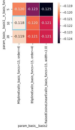
scikit-learn does not cache every model that it runs (that could get prohibitively large!), but it does store the best estimator, as the appropriately-named best_estimator_.

• Can easily grab the best estimator, the pipeline that did the best:

best_estim = cv.best_estimator_
best_estim

Pipeline(steps=[('basis',
                 Transformer(AdditiveBasis(
    basis1=MSplineEval(n_basis_funcs=10, order=4),
    basis2=MSplineEval(n_basis_funcs=15, order=4),
))),
                ('glm',
                 PopulationGLM(
    observation_model=PoissonObservations(inverse_link_function=exp),
    regularizer=UnRegularized(),
    solver_name='LBFGS',
    solver_kwargs={'tol': 1e-12}
))])

In a Jupyter environment, please rerun this cell to show the HTML representation or trust the notebook.
On GitHub, the HTML representation is unable to render, please try loading this page with nbviewer.org.

We then visualize the predictions of best_estim the same as before.

• Visualize model predictions!

visualize_model_predictions(best_estim, transformer_input)

/home/agent/workspace/rorse_ccn-software-jan-2025_main/lib/python3.11/site-packages/numpy/_core/fromnumeric.py:3904: RuntimeWarning: Mean of empty slice.
  return _methods._mean(a, axis=axis, dtype=dtype,
/home/agent/workspace/rorse_ccn-software-jan-2025_main/lib/python3.11/site-packages/numpy/_core/_methods.py:139: RuntimeWarning: invalid value encountered in divide
  ret = um.true_divide(

Feature selection

Now, finally, we understand almost enough about how scikit-learn works to figure out whether both position and speed are necessary inputs, i.e., to do feature selection. There’s just one more thing to learn: feature masks.

Each PopulationGLM object has a feature mask attribute, which allows us to exclude certain parts of the input. Its shape is X.shape[1] (number of columns in the design matrix) by n_neurons (number of neurons we’re trying to predict) and, if it’s not specified explicitly, a default mask including everything is created:

• Now one more thing we can do with scikit-learn!

• Each PopulationGLM object has a feature mask, which allows us to exclude certain parts of the input

• Feature mask shape: X.shape[1] (number of columns in the design matrix) by n_neurons (number of neurons we’re trying to predict)

• (By default, everything is included.)

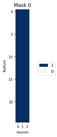
pipe['glm'].feature_mask
print(pipe['glm'].feature_mask.shape)

(25, 3)

workshop_utils.plot_feature_mask(pipe["glm"].feature_mask);

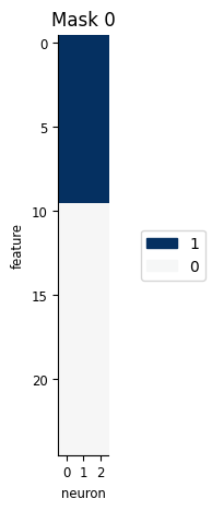
We could manually edit feature mask the feature mask, but we have some helper functions to help easily create them:

- We could manually edit feature mask, but have some helper functions -- these are currently being developed, so any feedback is appreciated! - By default, we include all features:

m = workshop_utils.create_feature_mask(pipe["basis"], n_neurons=count.shape[1])
workshop_utils.plot_feature_mask(m);

This function makes use of our additive basis to figure out the structure in the input and allows us to selectively remove some of the features:

• Make use of our additive basis to figure out the structure in the input

• Can selectively remove some of the features:

m = workshop_utils.create_feature_mask(pipe["basis"], ["all", "none"], n_neurons=count.shape[1])
fig=workshop_utils.plot_feature_mask(m);

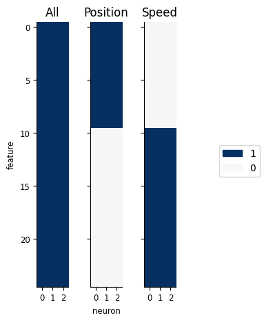
To perform feature selection, we’ll want to compare three masks: one including all inputs, one including just the position inputs, and one including just the speed inputs.

• Can construct a set of feature masks that includes / excludes each of the sets of inputs:

feature_masks = [
    workshop_utils.create_feature_mask(basis, "all", n_neurons=count.shape[1]),
    workshop_utils.create_feature_mask(basis, ["all", "none"], n_neurons=count.shape[1]),
    workshop_utils.create_feature_mask(basis, ["none", "all"], n_neurons=count.shape[1]),
]

workshop_utils.plot_feature_mask(feature_masks, ["All", "Position", "Speed"]);

One more wrinkle: the shape of this feature mask depends on the number of basis functions! (The number of features is basis.n_basis_funcs = basis.basis1.n_basis_funcs + basis.basis2.n_basis_funcs.) Thus we need to create a new feature mask for each possible arrangement. We do this in a helper function as well:

• One more wrinkle: the shape of this feature mask depends on the number of basis functions!

• Thus, must create a new feature mask for each possible arrangement:

param_grid = workshop_utils.create_feature_mask_paramgrid(basis, [5, 10, 20], 
                                                          [8, 16, 32], count.shape[1])

Now, as before, initialize and fit GridSearchCV:

• Initialize and fit GridSearchCV

cv = model_selection.GridSearchCV(best_estim, param_grid, cv=cv_folds)
cv.fit(transformer_input, count)

GridSearchCV(cv=5,
             estimator=Pipeline(steps=[('basis',
                                        Transformer(AdditiveBasis(
    basis1=MSplineEval(n_basis_funcs=10, order=4),
    basis2=MSplineEval(n_basis_funcs=15, order=4),
))),
                                       ('glm',
                                        PopulationGLM(
    observation_model=PoissonObservations(inverse_link_function=exp),
    regularizer=UnRegularized(),
    solver_name='LBFGS',
    solver_kwargs={'tol': 1e-12}
))]),
             param_grid=...
       [1., 1., 1.],
       [1., 1., 1.],
       [1., 1., 1.],
       [1., 1., 1.],
       [1., 1., 1.],
       [1., 1., 1.],
       [1., 1., 1.],
       [1., 1., 1.],
       [1., 1., 1.],
       [1., 1., 1.],
       [1., 1., 1.],
       [1., 1., 1.],
       [1., 1., 1.],
       [1., 1., 1.],
       [1., 1., 1.],
       [1., 1., 1.],
       [1., 1., 1.],
       [1., 1., 1.],
       [1., 1., 1.],
       [1., 1., 1.],
       [1., 1., 1.],
       [1., 1., 1.],
       [1., 1., 1.],
       [1., 1., 1.],
       [1., 1., 1.],
       [1., 1., 1.],
       [1., 1., 1.],
       [1., 1., 1.],
       [1., 1., 1.],
       [1., 1., 1.],
       [1., 1., 1.],
       [1., 1., 1.]])]}])

In a Jupyter environment, please rerun this cell to show the HTML representation or trust the notebook.
On GitHub, the HTML representation is unable to render, please try loading this page with nbviewer.org.

And examine the results:

• Investigate results using pandas

cv_df = pd.DataFrame(cv.cv_results_)
cv_df

	mean_fit_time	std_fit_time	mean_score_time	std_score_time	param_basis__basis1__n_basis_funcs	param_basis__basis2__n_basis_funcs	param_glm__feature_mask	params	split0_test_score	split1_test_score	split2_test_score	split3_test_score	split4_test_score	mean_test_score	std_test_score	rank_test_score
0	2.111473	0.298693	0.083012	0.083686	5	8	[[1.0, 1.0, 1.0], [1.0, 1.0, 1.0], [1.0, 1.0, ...	{'basis__basis1__n_basis_funcs': 5, 'basis__ba...	-0.115704	-0.105232	-0.139559	-0.119396	-0.117002	-0.119379	0.011194	7
1	2.186010	0.246932	0.092477	0.094525	10	8	[[1.0, 1.0, 1.0], [1.0, 1.0, 1.0], [1.0, 1.0, ...	{'basis__basis1__n_basis_funcs': 10, 'basis__b...	-0.114321	-0.104916	-0.139931	-0.118134	-0.117393	-0.118939	0.011504	5
2	2.273584	0.181114	0.098514	0.099149	20	8	[[1.0, 1.0, 1.0], [1.0, 1.0, 1.0], [1.0, 1.0, ...	{'basis__basis1__n_basis_funcs': 20, 'basis__b...	-0.114801	-0.105410	-0.141091	-0.119206	-0.116862	-0.119474	0.011780	8
3	2.195831	0.524363	0.014775	0.001161	5	8	[[0.0, 0.0, 0.0], [0.0, 0.0, 0.0], [0.0, 0.0, ...	{'basis__basis1__n_basis_funcs': 5, 'basis__ba...	-0.152824	-0.123502	-0.156398	-0.130596	-0.133044	-0.139273	0.012960	13
4	2.255210	0.204189	0.105998	0.110213	5	16	[[0.0, 0.0, 0.0], [0.0, 0.0, 0.0], [0.0, 0.0, ...	{'basis__basis1__n_basis_funcs': 5, 'basis__ba...	-0.154570	-0.124092	-0.156435	-0.130892	-0.133329	-0.139864	0.013136	14
5	2.242129	0.301981	0.119251	0.122137	5	32	[[0.0, 0.0, 0.0], [0.0, 0.0, 0.0], [0.0, 0.0, ...	{'basis__basis1__n_basis_funcs': 5, 'basis__ba...	-0.157214	-0.124906	-0.161839	-0.131216	-0.138397	-0.142714	0.014450	15
6	1.770313	0.040023	0.013384	0.000698	5	8	[[1.0, 1.0, 1.0], [1.0, 1.0, 1.0], [1.0, 1.0, ...	{'basis__basis1__n_basis_funcs': 5, 'basis__ba...	-0.112460	-0.105061	-0.142699	-0.118276	-0.116293	-0.118958	0.012701	6
7	2.289364	0.715357	0.016018	0.001157	5	16	[[1.0, 1.0, 1.0], [1.0, 1.0, 1.0], [1.0, 1.0, ...	{'basis__basis1__n_basis_funcs': 5, 'basis__ba...	-0.116043	-0.105530	-0.141566	-0.118699	-0.117384	-0.119844	0.011820	9
8	2.273666	0.031797	0.022941	0.000863	5	32	[[1.0, 1.0, 1.0], [1.0, 1.0, 1.0], [1.0, 1.0, ...	{'basis__basis1__n_basis_funcs': 5, 'basis__ba...	-0.123822	-0.106465	-0.147354	-0.119323	-0.121296	-0.123652	0.013278	12
9	1.958681	0.073457	0.014907	0.001000	10	8	[[1.0, 1.0, 1.0], [1.0, 1.0, 1.0], [1.0, 1.0, ...	{'basis__basis1__n_basis_funcs': 10, 'basis__b...	-0.112012	-0.103949	-0.141152	-0.116966	-0.115391	-0.117894	0.012467	1
10	2.190175	0.283126	0.136258	0.147648	10	16	[[1.0, 1.0, 1.0], [1.0, 1.0, 1.0], [1.0, 1.0, ...	{'basis__basis1__n_basis_funcs': 10, 'basis__b...	-0.113170	-0.104628	-0.141212	-0.117088	-0.115814	-0.118382	0.012213	2
11	2.559328	0.330215	0.160526	0.170735	10	32	[[1.0, 1.0, 1.0], [1.0, 1.0, 1.0], [1.0, 1.0, ...	{'basis__basis1__n_basis_funcs': 10, 'basis__b...	-0.117302	-0.105385	-0.145113	-0.117099	-0.119184	-0.120817	0.013094	10
12	2.660137	0.859940	0.017878	0.001070	20	8	[[1.0, 1.0, 1.0], [1.0, 1.0, 1.0], [1.0, 1.0, ...	{'basis__basis1__n_basis_funcs': 20, 'basis__b...	-0.112046	-0.104498	-0.142396	-0.118190	-0.115020	-0.118430	0.012813	3
13	2.553034	0.353206	0.156188	0.163277	20	16	[[1.0, 1.0, 1.0], [1.0, 1.0, 1.0], [1.0, 1.0, ...	{'basis__basis1__n_basis_funcs': 20, 'basis__b...	-0.112752	-0.104975	-0.142423	-0.118130	-0.115327	-0.118721	0.012635	4
14	2.580529	0.341920	0.173372	0.182261	20	32	[[1.0, 1.0, 1.0], [1.0, 1.0, 1.0], [1.0, 1.0, ...	{'basis__basis1__n_basis_funcs': 20, 'basis__b...	-0.116874	-0.105859	-0.147083	-0.118258	-0.119202	-0.121455	0.013684	11

• For our own sanity, let’s create an easier-to-read label:

# create a custom label to make the results easier to parse
def label_feature_mask(x):
    mask = x.param_glm__feature_mask
    if mask.sum() / np.prod(mask.shape) == 1:
        return "all"
    elif mask[0,0] == 1:
        return "position"
    else:
        return "speed"

cv_df['feature_mask_label'] = cv_df.apply(label_feature_mask, 1)

• And visualize:

workshop_utils.plot_heatmap_cv_results(cv_df, "feature_mask_label", columns="param_basis__basis2__n_basis_funcs")

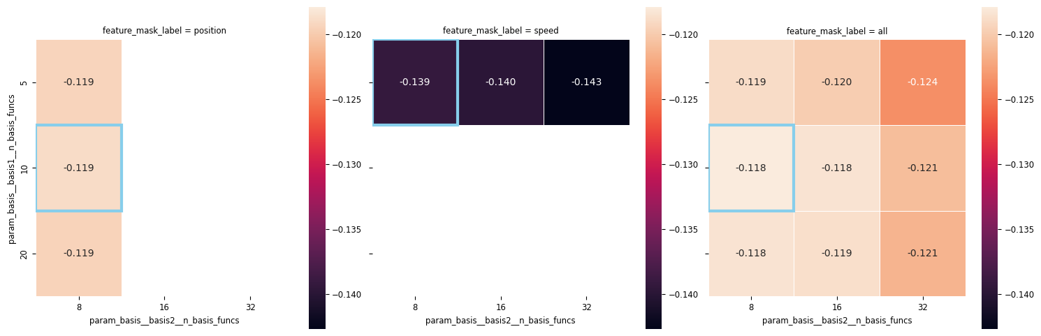
• What do we see?

From the above plots, we can see that:

• Position matters more than speed.

• Number of basis functions for speed doesn’t matter much.

• We don’t need many basis functions to represent the position.

From the above plots, we can see that:

• Position matters more than speed.

• Number of basis functions for speed doesn’t matter much.

• We don’t need many basis functions to represent the position.

Let’s visualize the predictions of the best estimator.

• Visualize model predictions!

visualize_model_predictions(cv.best_estimator_, transformer_input)

/home/agent/workspace/rorse_ccn-software-jan-2025_main/lib/python3.11/site-packages/numpy/_core/fromnumeric.py:3904: RuntimeWarning: Mean of empty slice.
  return _methods._mean(a, axis=axis, dtype=dtype,
/home/agent/workspace/rorse_ccn-software-jan-2025_main/lib/python3.11/site-packages/numpy/_core/_methods.py:139: RuntimeWarning: invalid value encountered in divide
  ret = um.true_divide(

Conclusion

Various combinations of features can lead to different results. Feel free to explore more. To go beyond this notebook, you can check the following references :

• Hardcastle, Kiah, et al. “A multiplexed, heterogeneous, and adaptive code for navigation in medial entorhinal cortex.” Neuron 94.2 (2017): 375-387

• McClain, Kathryn, et al. “Position–theta-phase model of hippocampal place cell activity applied to quantification of running speed modulation of firing rate.” Proceedings of the National Academy of Sciences 116.52 (2019): 27035-27042

• Peyrache, Adrien, Natalie Schieferstein, and Gyorgy Buzsáki. “Transformation of the head-direction signal into a spatial code.” Nature communications 8.1 (2017): 1752.

References

The data in this tutorial comes from Grosmark, Andres D., and György Buzsáki. “Diversity in neural firing dynamics supports both rigid and learned hippocampal sequences.” Science 351.6280 (2016): 1440-1443.