Matsubara fitting for data with continuous spectrum (semicircular density)
In this notebook, we aim to fit the following Matsubara function:
where \(\rho(w)\) is the semicircular spectral function
and \(\mathrm i\nu_n\) is the Matsubara frequency:
Here \(\beta\) is the inverse temperature.
Let us first set inverse temperature \(\beta\) and the Matsubara frequencies \(Z = \{\mathrm i\nu_n\}\).
import numpy as np
import matplotlib.pyplot as plt
from adapol import hybfit
import scipy
beta = 20
N = 55
Z = 1j *(np.linspace(-N, N, N + 1)) * np.pi / beta
Now we construct the Matsubara data using the above equation. The integral is evaluated with adaptive quadrature:
def Kw(w, v):
    return 1 / ( v - w)
def semicircular(x):
    return 2 * np.sqrt(1 - x**2) / np.pi
def make_Delta_with_cont_spec( Z, rho, a=-1.0, b=1.0, eps=1e-12):
    Delta = np.zeros((Z.shape[0]), dtype=np.complex128)
    for n in range(len(Z)):
        def f(w):
            return Kw(w , Z[n]) * rho(w)

        # f = lambda w: Kw(w-en[i],Z[n])*rho(w)
        Delta[n] = scipy.integrate.quad(
            f, a, b, epsabs=eps, epsrel=eps, complex_func=True
        )[0]


    return Delta

Delta = make_Delta_with_cont_spec( Z, semicircular)
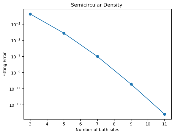
Below we show that by increasing number of modes \(N_p\), the fitting error decreases.
error = []
Nbath = []
for Np in range(2, 12, 2):
    bathenergy, bathhyb, final_error, func = hybfit(Delta, Z, Np = Np, verbose=False)
    Nbath.append(len(bathenergy))
    error.append(final_error)
plt.yscale('log')
plt.plot(Nbath, error, 'o-')
plt.xlabel('Number of bath sites')
plt.ylabel('Fitting Error')
plt.title("Semicircular Density ")
plt.show()
Triqs Interface
Let us demonstrate how to use our code if the Matsubara functions are given using the TRIQS data structure.
In trqis, the Matsubara frequencies are defined using MeshImFreq:
from triqs.gf import MeshImFreq
Norb = 1
iw_mesh = MeshImFreq(beta=beta, S='Fermion', n_iw=Z.shape[0]//2)
The hybfit_triqs function could handle TRIQS Green’s functions
object GF and BlockGf:
from triqs.gf import Gf, BlockGf
from adapol import hybfit_triqs
delta_iw = Gf(mesh=iw_mesh, target_shape=[Norb, Norb])
delta_iw.data[:,0,0] = Delta

#Construct BlockGf object
delta_blk = BlockGf(name_list=['up', 'down'], block_list=[delta_iw, delta_iw], make_copies=True)

tol = 1e-6
# Gf interface for hybridization fitting
bathhyb, bathenergy, delta_fit, final_error = hybfit_triqs(delta_iw, tol=tol, maxiter=50, debug=True)
assert final_error < tol

# BlockGf interface for hybridization fitting
bathhyb, bathenergy, delta_fit, final_error = hybfit_triqs(delta_blk, tol=tol, maxiter=50, debug=True)
assert final_error[0] < tol and final_error[1] < tol
optimization finished with fitting error 9.538e-08
optimization finished with fitting error 9.538e-08
optimization finished with fitting error 9.538e-08