Matsubara fitting for data generated by discrete poles
In this note, let us illustrate how to perform Matsubara fitting using test data generated by discrete poles with random weights.
Let us first define the inverse temperature \(\beta\) and Matsubara frequencies \(\{Z_n\}\):
import numpy as np
import matplotlib.pyplot as plt
from adapol import hybfit

beta = 20
N = 55
Z = 1j *(np.linspace(-N, N, N + 1)) * np.pi / beta
We will generate Matsubara data evaluated on \(\{Z_n\}\) using the following formula:
Where \(|v_k\rangle\) is a \(N_{\text{orb}}\times 1\) vector, where \(N_{\text{orb}}\) is the number of orbitals.
Below is the code for making a \(N_{\text{orb}}\)-dimensional Matsubara data on Matsubara frequencies \(Z\), by summing with \(N_p\) discrete poles.
def make_Delta_with_random_discrete_pole(Norb, Np, Z):
    np.random.seed(0)
    pol = np.cos((2*np.arange(Np)+1) * np.pi / (2*Np) )
    vec = np.random.randn(Norb, Np) + 1j * np.random.randn(Norb, Np)
    weight = np.array(
        [vec[:, i, None] * np.transpose(np.conj(vec[:, i])) for i in range(Np)]
    )

    pol_t = np.reshape(pol, [pol.size, 1])
    M = 1 / ( Z - pol_t)
    M = M.transpose()
    if len(weight.shape) == 1:
        weight = weight / sum(weight)
        Delta = M @ weight
    else:
        Nw = len(Z)
        Delta = (M @ (weight.reshape(Np, Norb * Norb))).reshape(Nw, Norb, Norb)
    return pol, weight, Delta
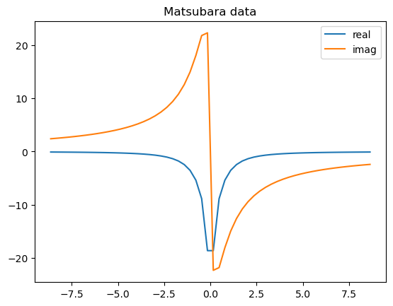
An example Matsubara data would look like the following:
pol, weight, Delta = make_Delta_with_random_discrete_pole(Norb=1, Np = 10, Z=Z)

plt.plot(Z.imag, Delta[:, 0, 0].real, label='real')
plt.plot(Z.imag, Delta[:, 0, 0].imag, label='imag')
plt.legend()
plt.title("Matsubara data")
Text(0.5, 1.0, 'Matsubara data')
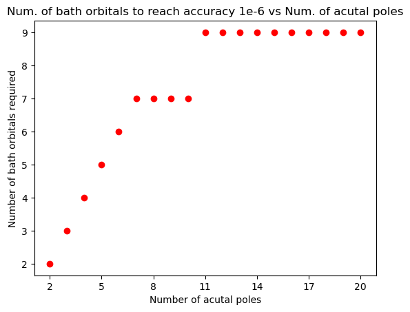
Let us first test the Matsubara fitting for scalar-valued Matsubara functions.
tol = 1e-6 #Fitting tolerance

for Np in range(2, 21):
    pol, weight, Delta = make_Delta_with_random_discrete_pole(Norb=1, Np = Np, Z=Z)
    bathenergy, bathhyb, final_error, func = hybfit(Delta, Z, tol=tol)
    assert(final_error < tol)
    plt.plot(Np, len(bathenergy),"ro")
plt.xlabel("Number of acutal poles")
plt.ylabel("Number of bath orbitals required")
plt.title("Num. of bath orbitals to reach accuracy 1e-6 vs Num. of acutal poles")
plt.xticks(range(2, 21,3))
plt.show()
Similarly, we can test for matrix-valued Matsubara functions:
tol = 1e-6
Norb = 4

for Np in range(2, 10):
    pol, weight, G = make_Delta_with_random_discrete_pole(Norb=Norb, Np = Np, Z=Z)
    bathenergy, bathhyb, final_error, func = hybfit(G, Z, tol=tol)
    assert(final_error < tol)
One can also conduct Matsubara fitting via specifying number of modes \(N_p\) in the hybfit function:
pol, weight, G = make_Delta_with_random_discrete_pole(Norb=4, Np = 10, Z=Z)
bathenergy, bathhyb, final_error, func = hybfit(G, Z, Np=15)
print("Numer of bath orbitals is ", len(bathenergy))
print("Final error is ", final_error)
Numer of bath orbitals is  10
Final error is  6.189103600097627e-10
Triqs Interface
Let us demonstrate how to use our code if the Matsubara functions are given using the TRIQS data structure.
In trqis, the Matsubara frequencies are defined using MeshImFreq:
from triqs.gf import MeshImFreq
Norb = 1
iw_mesh = MeshImFreq(beta=beta, S='Fermion', n_iw=Z.shape[0]//2)
The hybfit_triqs function could handle TRIQS Green’s functions
object GF and BlockGf:
from triqs.gf import Gf, BlockGf
from adapol import hybfit_triqs
Norb = 1
for Np in range(2, 21):
    pol, weight, Delta = make_Delta_with_random_discrete_pole(Norb=Norb, Np = Np, Z=Z)

    #Construct Gf object
    delta_iw = Gf(mesh=iw_mesh, target_shape=[Norb, Norb])
    delta_iw.data[:] = Delta

    #Construct BlockGf object
    delta_blk = BlockGf(name_list=['up', 'down'], block_list=[delta_iw, delta_iw], make_copies=True)

    # Gf interface for hybridization fitting
    bathhyb, bathenergy, delta_fit, final_error = hybfit_triqs(delta_iw, tol=tol, maxiter=50, debug=True)
    assert final_error < tol

    # BlockGf interface for hybridization fitting
    bathhyb, bathenergy, delta_fit, final_error = hybfit_triqs(delta_blk, tol=tol, maxiter=50, debug=True)
    assert final_error[0] < tol and final_error[1] < tol
optimization finished with fitting error 2.701e-15
optimization finished with fitting error 2.701e-15
optimization finished with fitting error 2.701e-15
optimization finished with fitting error 1.081e-14
optimization finished with fitting error 1.081e-14
optimization finished with fitting error 1.081e-14
optimization finished with fitting error 1.099e-14
optimization finished with fitting error 1.099e-14
optimization finished with fitting error 1.099e-14
optimization finished with fitting error 2.220e-14
optimization finished with fitting error 2.220e-14
optimization finished with fitting error 2.220e-14
optimization finished with fitting error 2.892e-14
optimization finished with fitting error 2.892e-14
optimization finished with fitting error 2.892e-14
optimization finished with fitting error 1.905e-14
optimization finished with fitting error 1.905e-14
optimization finished with fitting error 1.905e-14
optimization finished with fitting error 4.401e-07
optimization finished with fitting error 4.401e-07
optimization finished with fitting error 4.401e-07
optimization finished with fitting error 7.920e-08
optimization finished with fitting error 7.920e-08
optimization finished with fitting error 7.920e-08
optimization finished with fitting error 7.742e-07
optimization finished with fitting error 7.742e-07
optimization finished with fitting error 7.742e-07
optimization finished with fitting error 1.444e-10
optimization finished with fitting error 1.444e-10
optimization finished with fitting error 1.444e-10
optimization finished with fitting error 2.079e-09
optimization finished with fitting error 2.079e-09
optimization finished with fitting error 2.079e-09
optimization finished with fitting error 7.408e-10
optimization finished with fitting error 7.408e-10
optimization finished with fitting error 7.408e-10
optimization finished with fitting error 1.092e-09
optimization finished with fitting error 1.092e-09
optimization finished with fitting error 1.092e-09
optimization finished with fitting error 2.791e-09
optimization finished with fitting error 2.791e-09
optimization finished with fitting error 2.791e-09
optimization finished with fitting error 1.611e-09
optimization finished with fitting error 1.611e-09
optimization finished with fitting error 1.611e-09
optimization finished with fitting error 1.047e-09
optimization finished with fitting error 1.047e-09
optimization finished with fitting error 1.047e-09
optimization finished with fitting error 1.827e-09
optimization finished with fitting error 1.827e-09
optimization finished with fitting error 1.827e-09
optimization finished with fitting error 3.379e-09
optimization finished with fitting error 3.379e-09
optimization finished with fitting error 3.379e-09
optimization finished with fitting error 1.989e-09
optimization finished with fitting error 1.989e-09
optimization finished with fitting error 1.989e-09