Examples
This page gives one step-by-step example of the most basic usage of the DLR
within cppdlr. For a basic overview of the DLR, definitions, and
conventions, please see the background page.
Further examples, containing thorough documentation of all steps, can be
found in the examples directory of the repository. The list of
examples below gives a list of all examples, with brief
descriptions. These examples should serve as a good starting point for writing
your own code using cppdlr.
For the time being, not all use cases are covered by examples in the
examples directory. However, the test directory of the repository
contains tests of all the components of cppdlr, and these can also serve as
useful examples (though they might not be as user-friendly as the examples in
the examples directory). Therefore, in the list of other
capabilities below, we list capabilities of cppdlr
which are not currently covered by examples, and point to the relevant tests in
the test directory which can serve as examples of these capabilities. This
is a temporary measure, until we have a more comprehensive set of examples.
Example: form a DLR expansion via interpolation, and evaluate it in imaginary time and frequency
This example follows the example program in the file
examples/dlr_interpolation.cpp. You should follow the code in that file as
you read this example. If you see a definition you do not know, or need to look
up a convention, you can find this information on the background page.
We first include the header file cppdlr.hpp, which is
necessary to use cppdlr functionality, and use the cppdlr namespace. We
then define an evaluator function, gfun, for an imaginary time Green’s
function. In this case, we take a simple example: a Green’s function
corresponding to a spectral function which is a discrete sum of delta functions:
In this case, we have taken each \(A_i\) to be a \(2 \times 2\) symmetric matrix. Using the Lehmann representation, defined on the background page, we see that this yields the following imaginary time Green’s function:
There is nothing special about this Green’s function, except that it is convenient for this example because it has a simple analytical form. We also define an evaluator for the Green’s function in fermionic Matsubara frequency space, which, by direct Fourier transform, is given by
Next we move to the main program. We first define the the inverse temperature \(\beta\), the number of orbital indices, which in this case is 2 since \(G\) is a \(2 \times 2\) matrix-valued function, the DLR cutoff parameter \(\Lambda\), and the desired accuracy \(\epsilon\) of our DLR expansion. We note that we took all the \(a_i\) above to be less than 1, so the spectral width \(\omega_{\max}\) of the Green’s function is less than 1; therefore, the DLR cutoff parameter \(\Lambda = \beta \omega_{\max}\) can be safely set to \(\beta\). If the spectral width is unknown, it is recommended to converge results with respect to \(\Lambda\). After this, we set the number of points at which we will test the accuracy of our DLR expansion, both in imaginary time and Matsubara frequency.
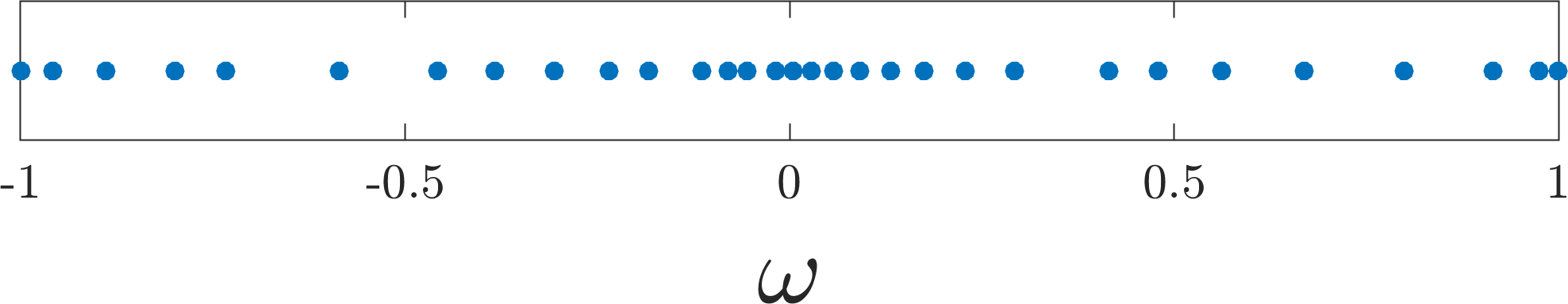
We now begin to see some of the basic functionality of cppdlr. We first
obtain the DLR frequencies \(\omega_l\) by calling the function
build_dlr_rf, supplying the DLR cutoff parameter and tolerance as input
parameters. We obtain a vector of \(r = 31\) DLR frequencies, which are
shown below for the given parameters. We note that although cppdlr works in
non-dimensionalized variables (e.g., we consider \(\tau \in [0,1]\) rather
than \(\tau \in [0,\beta]\)), we have converted back to the original
physical variables in all figures on this page.
We next obtain an object of type imtime_ops. This class is responsible for
all imaginary time operations on Green’s functions, such as interpolation,
fitting, and convolution, and given a particular set of DLR frequencies,
determined by \(\Lambda\) and \(\epsilon\), you only need one of these.
The vector of DLR imaginary time grid nodes \(\tau_k\) can be extracted from
this object using the get_itnodes method.
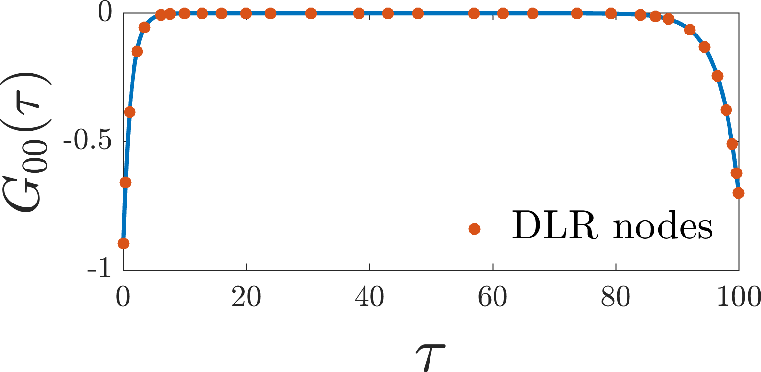
We next evaluate the Green’s function at the DLR imaginary time grid nodes by calling the evaluator function discussed above. In practice, you would supply your own Green’s function evaluator, which could involve a complicated program. Below, we plot the Green’s function, with the \(r = 31\) DLR imaginary time nodes indicated.
Now that we have the values of the Green’s function on the DLR imaginary time
grid, \(G(\tau_k)\), we can form its DLR expansion by obtaining its DLR
coefficients \(\widehat{g}_l\) via the vals2coefs method of the
imtime_ops object. We sometimes call this the interpolation step, since we
are interpolating the Green’s function at the DLR nodes using an expansion in
the DLR basis functions \(K(\tau, \omega_l)\). In other words, we solve the
linear system
which constitutes an interpolation problem.
Having obtained the DLR expansion of \(G\) (characterized by its DLR coefficients \(\widehat{g}_l\)), we can now evaluate it at any imaginary time point \(\tau\) by simply evaluating the DLR expansion:
This is done using the coefs2eval method of the imtime_ops object. Here,
we evaluate the DLR expansion on an equispaced grid of \(\tau\) points
generated by the function eqptsrel (this function generates the points in
the relative time format used by cppdlr; please see the imaginary
time point format section of the Background page for details). We also evaluate
the true Green’s function, and compare the two. The pointwise error for the
top-left entry of the Green’s function, \(G_00(\tau)\), is shown below.
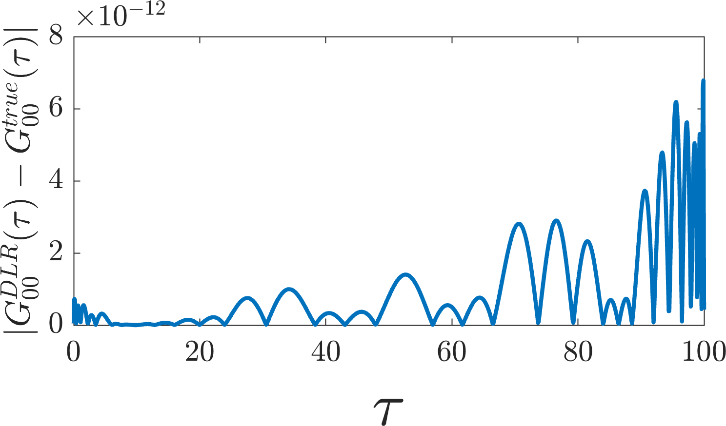
We see that the DLR expansion is correct to within the specified \(\epsilon = 10^{-10}\) tolerance.
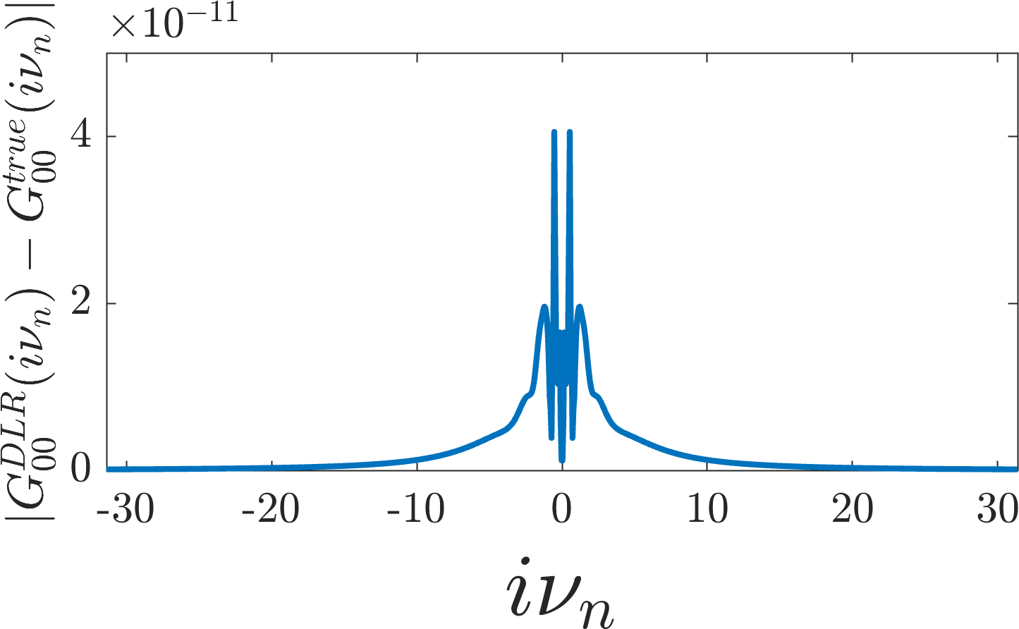
Since the Fourier transform of the DLR basis functions are known, we can directly evaluate the DLR expansion of \(G\) in the fermionic Matsubara frequency space:
To do this, we first construct an object of type imfreq_ops. This class is
analogous to the imtime_ops class, but is responsible for all Matsubara
frequency operations. Here, we use its coefs2eval method to evaluate the DLR
expansion of \(G\) at a large set of Matsubara frequencies, which in cppdlr
are characterized by their index \(n\). Again comparing to the top-left
entry \(G_00(i \nu_n)\) of the true Green’s
function, we find agreement within the specified \(\epsilon = 10^{-10}\)
tolerance.
List of examples
The examples directory contains the following example programs, which are
documented in detail in the files themselves.
examples/dlr_interpolation.cpp: form a DLR expansion via interpolation, and evaluate it in imaginary time and frequency. This example is described in detail above.
List of other cppdlr capabilities
For cppdlr use cases which are not covered by examples in the examples directory,
relevant unit tests in the test directory can serve as useful examples. We
list several such use cases below.
Obtain a DLR expansion by fitting to data in imaginary time: see the tests
imtime_ops.fit_scalar,imtime_ops.fit_matrix, andimtime_ops.fit_matrix_cmplxin the filetest/imtime_ops.cpp.Compute the convolution of two DLR expansions: see the tests
imtime_ops.convolve_scalar_real,imtime_ops.convolve_scalar_cmplx,imtime_ops.convolve_matrix_real, andimtime_ops.convolve_matrix_cmplxin the filetest/imtime_ops.cpp.Perform a “reflection” operation \(G(\tau) \mapsto G(\beta-\tau)\) on a Green’s function: see the test
imtime_ops.refl_matrixin the filetest/imtime_ops.cpp.Compute the inner product of two DLR expansions: see the test
imtime_ops.innerprodin the filetest/imtime_ops.cpp.Obtain a DLR expansion by interpolation on the DLR Matsubara frequency nodes: see the tests
imfreq_ops.interp_scalarandimfreq_ops.interp_matrixin the filetest/imfreq_ops.cpp.Obtain symmetrized DLR grids, and obtain a DLR expansion by interpolation on these grids: see the tests
imtime_ops.interp_matrix_sym_ferandimtime_ops.interp_matrix_sym_bosin the filetest/imtime_ops.cppfor fermionic and bosonic Green’s functions, respectively, on a symmetric imaginary time grid. See the testsimfreq_ops.interp_matrix_sym_ferandimfreq_ops.interp_matrix_sym_bosin the filetest/imfreq_ops.cppfor fermionic and bosonic Green’s functions, respectively, on a symmetric Matsubara frequency grid. All of these tests show how to obtain a symmetric set of DLR frequencies.Given a fixed self-energy, solve the Dyson equation in imaginary time to obtain the Green’s function: see the tests
dyson_it.dyson_vs_ed_real,dyson_it.dyson_vs_ed_cmplx, anddyson_it.dyson_bethein the filetest/dyson_it.cpp.Solve the Dyson equation self-consistently in imaginary time, given an expression for the self-energy in terms of the Green’s function: see the test
dyson_it.dyson_bethe_fpiin the filetest/dyson_it.cpp.