Analytic continuation of Hubbard dimer

In this notebook, we illustrate how to conduct analytic continuation using adapol, using the strongly correlated Hubbard dimer model as an example. On the one hand, it serves as a nontrivial, challenging test case, featuring several closely-spaced peaks in the spectrum. On the other hand, its modest size allows for exact diagonalization, enabling the calculation of ground truth results for rigorous benchmarking. This example was also used as a benchmark test in this and this paper.

Let us consider the following Hamiltonian:

\[\hat H = \hat H_0 + \hat H_1,\]

where

\[H_0 = -t \sum_{\sigma \in \{\uparrow, \downarrow\}} \left( \hat c_{0\sigma}^\dagger \hat c_{1\sigma} + \hat c_{1\sigma}^\dagger \hat c_{0\sigma} \right) -\mu \left( \hat n_{0\uparrow} + \hat n_{0\downarrow} + \hat n_{1\uparrow} + \hat n_{1\downarrow} \right),\]

\[\begin{split}\begin{aligned} H_1 =& (U+U_a) \hat n_{0\uparrow} \hat n_{0\downarrow} + (U-U_a) \hat n_{1\uparrow} \hat n_{1\downarrow} \\ & - \frac U 2 \left( \hat n_{0\uparrow} + \hat n_{0\downarrow} + \hat n_{1\uparrow} + \hat n_{1\downarrow} \right) + h \left( \hat n_{0\uparrow} - \hat n_{0\downarrow} + \hat n_{1\uparrow} - \hat n_{1\downarrow} \right)\\ &+ \mu_a \left( \hat n_{0\uparrow} + \hat n_{0\downarrow} - \hat n_{1\uparrow} - \hat n_{1\downarrow} \right)+ h_a \left( \hat n_{0\uparrow} - \hat n_{0\downarrow} - \hat n_{1\uparrow} + \hat n_{1\downarrow} \right), \end{aligned}\end{split}\]

Here \(\hat n_{i\sigma} = \hat c_{i\sigma}^\dagger \hat c_{i\sigma}\) is the number operator.

The parameters are taken as follows:

from triqs.operators import c, c_dag,n
from triqs.atom_diag import AtomDiag, atomic_g_w, atomic_g_iw
from itertools import product
import matplotlib.pyplot as plt
import numpy as np

t = 1.0
mu = 0.7
h = 0.3
U_a = 0.5
mu_a = 0.2
h_a = 0.03
beta = 25.0
U = 5.0

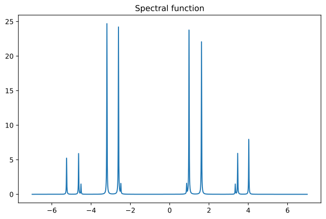
Using triqs, we can construct the Hamiltonian and obtain the Green’s function and spectral function through exact diagonalization:

f_ops = [(sn,on) for sn, on in product(('up','down'),range(2))]
H_0 = - t * (c_dag('up', 0) * c('up', 1) + c_dag('up', 1) * c('up', 0) )
H_0 += - t * (c_dag('down', 0) * c('down', 1) + c_dag('down', 1) * c('down', 0) )
H_0 += - mu * (n('up', 0) + n('down', 0)) - mu * (n('up', 1) + n('down', 1))

H_1 = (U + U_a) * (n('up', 0) * n('down', 0) ) + (U - U_a) * (n('up', 1) * n('down', 1) )
H_1 -= (U/2.0) * (n('up', 0) + n('down', 0)  + n('up', 1) + n('down', 1) )
H_1 += h * (n('up', 0) - n('down', 0) + n('up', 1) - n('down', 1) )
H_1 += mu_a * (n('up', 0) + n('down', 0) - n('up', 1) - n('down', 1) )
H_1 += h_a * (n('up', 0) - n('down', 0) - n('up', 1) + n('down', 1) )

H = H_0 + H_1
ad = AtomDiag(H, f_ops)

gf_struct = [('down',2),('up',2)] # fix the bug in the old version by changing orb_names to len(orb_names).
G_w = atomic_g_w(ad, beta, gf_struct, (-7, 7), 4000, 0.01)
Tr_G_w = G_w['up'][0,0] + G_w['down'][0,0] + G_w['up'][1,1] + G_w['down'][1,1]
wmesh = np.array([w.value for w in Tr_G_w.mesh])
plt.plot(wmesh,  -np.imag(Tr_G_w.data)/np.pi)
plt.title("Spectral function")
plt.show()

Let us also construct the Matsubara Green’s function data:

G_iw = atomic_g_iw(ad, beta, gf_struct, 500)
TrG_iw = G_iw['up'][0,0] + G_iw['down'][0,0] + G_iw['up'][1,1] + G_iw['down'][1,1]
iwmesh = np.array([iw.value.value for iw in TrG_iw.mesh])

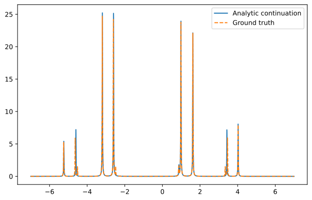
We perform analytic continuation by broadening the sum-of-delta functions representation of the spectral function produced by adapol:

from adapol import approx_freq_aaa
from adapol.sop import SumOfSimplePoles

poles, residues, err = approx_freq_aaa(TrG_iw.data, iwmesh, max_n_poles=12)
sop = SumOfSimplePoles(poles=poles, residues=residues)
Spec_approx = -np.imag(sop(wmesh+0.01*1j))/np.pi

plt.plot(wmesh,  Spec_approx)
plt.plot(wmesh,  -np.imag(Tr_G_w.data)/np.pi,  "--",2)
plt.legend(["Analytic continuation", "Ground truth"])
plt.show()

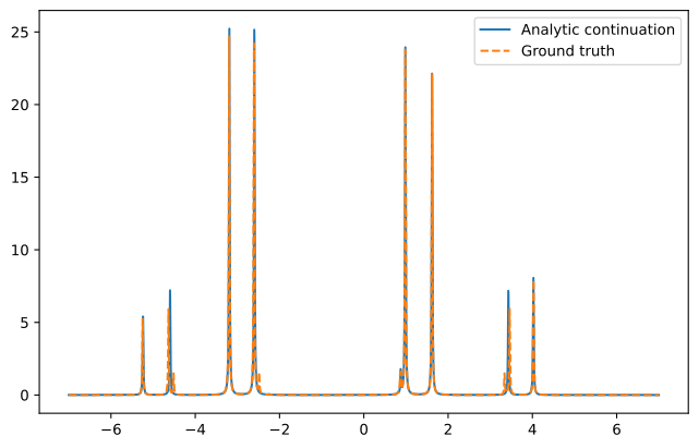
We can do the same using the triqs interface:

from adapol.triqs import approx_gf_imfreq_aaa

poles, residues, err = approx_gf_imfreq_aaa(TrG_iw, max_n_poles=12)
sop2 = SumOfSimplePoles(poles=poles, residues=residues)
Spec_approx2 = -np.imag(sop2(wmesh+0.01*1j))/np.pi

plt.plot(wmesh,  Spec_approx2)
plt.plot(wmesh,  -np.imag(Tr_G_w.data)/np.pi,  "--",2)
plt.legend(["Analytic continuation", "Ground truth"])
plt.show()